Portable vLLM Model Inference Kernels in Helion
10 Jun 2026, 5:00 pmTL;DR
Helion kernels were integrated into vLLM for FP8 inference using Qwen3 models and evaluated across NVIDIA H100 and B200 GPUs. The experiments show that Helion provides a productive PyTorch-native workflow for developing fused GPU kernels while delivering performance improvements for many quantization, normalization, and fusion-heavy inference kernels. End-to-end benchmarks demonstrated throughput gains across multiple serving scenarios, with additional optimization work underway for GEMM performance on Blackwell GPUs.
Brief Background on vLLM and Helion
vLLM is a high-performance inference and serving framework for large language models (LLMs). It is widely used for production LLM serving due to its strong throughput performance, efficient KV-cache management, continuous batching architecture, and support for advanced inference features such as speculative decoding, quantization, and distributed serving. Internally, vLLM relies heavily on custom GPU kernels, TorchInductor fusion, and optimized GEMM backends such as CUTLASS and DeepGEMM to achieve high inference efficiency across different hardware platforms.
Helion is a PyTorch-native hardware agnostic kernel DSL designed for writing high-performance kernels using a tile-programming model. Unlike lower-level CUDA programming, Helion provides a more natural PyTorch-syntax-centric development experience while still exposing low-level control over memory layout, tiling strategy, and kernel scheduling. You can think of it as PyTorch with tiles. If you know PyTorch or Triton, you already know most of Helion. Other than smooth authoring experience, another strength of Helion is its powerful ahead-of-time (AOT) autotuning infrastructure, which can explore a large kernel configuration space and automatically select optimized implementations for specific workloads and hardware targets.
vLLM Model Inference with Helion Kernels
We began by focusing on tensor-parallel-free inference using the Qwen3 model family with FP8 activation quantization enabled.
Our goal was to evaluate whether Helion kernels can improve inference performance compared to the existing vLLM implementations.
For this experiment, we replaced nearly all forward-pass kernels involved in quantized inference with Helion implementations and benchmarked them at both kernel level and end-to-end serving level.
vLLM Forward Pass Fusion Pattern
For Qwen3 models, the unfused forward pass in vLLM executes the following sequence of kernels:
- input_norm
- fp8_quant
- scaled_mm (qkv_proj)
- split_qkv
- q_norm
- k_norm
- rope
- attention
- fp8_quant
- scaled_mm (out_proj)
- post_attention_norm
- fp8_quant
- scaled_mm (gate_up)
- silu_and_mul
- fp8_quant
- scaled_mm (down_proj)
Dynamic Per-Token Activation Quantization
After torch.compile and TorchInductor fusion passes are applied, the execution pattern becomes:
- rms_norm + fp8_quant
- scaled_mm (qkv_proj)
- split_qkv + q_norm + v_norm
- rope
- attention
- fp8_quant
- scaled_mm (out_proj)
- rms_norm + fp8_quant
- scaled_mm (gate_up)
- silu_and_mul + fp8_quant
- scaled_mm (down_proj)
Note that both scaled_mm and attention are registered as PyTorch Custom Operators. Since these operators are opaque to TorchInductor, they form hard boundaries that prevent further compiler-side fusion.
Dynamic Per-Group Activation Quantization
When dynamic per-group activation quantization is enabled and DeepGEMM is selected for scaled_mm_blockwise, the execution pattern changes to:
- rms_norm
- fp8_quant (ue8m0)
- scaled_mm (qkv_proj, DeepGEMM)
- split_qkv + q_norm + v_norm
- rope
- attention
- fp8_quant (ue8m0)
- scaled_mm (out_proj, DeepGEMM)
- rms_norm
- fp8_quant (ue8m0)
- scaled_mm (gate_up, DeepGEMM)
- silu_and_mul
- fp8_quant (ue8m0)
- scaled_mm (down_proj, DeepGEMM)
DeepGEMM uses UE8M0 activation quantization internally. In the current vLLM implementation, fuse_act_quant and fuse_norm_quant passes are not supported for UE8M0 quantization, which prevents these additional fusions from occurring.
If DeepGEMM is unavailable and CUTLASS-based kernels are used instead, the execution pattern becomes similar to the dynamic per-token quantization case.
Helion Kernels Implementation
For this work, we implemented the following Helion kernels:
- dynamic_per_token_scaled_fp8_quant
- rms_norm_dynamic_per_token_quant
- silu_and_mul_dynamic_per_token_quant
- fused_qk_norm_rope
- per_token_group_fp8_quant
- rms_norm_per_block_quant
- silu_and_mul_per_block_quant
- scaled_mm
- scaled_mm_blockwise
The scaled_mm and scaled_mm_blockwise kernels follow the existing Triton implementations in vLLM (triton_scaled_mm, w8a8_triton_block_scaled_mm). silu_and_mul_dynamic_per_token_quant is a new fused kernel that combines silu_and_mul and dynamic_per_token_quant into a single kernel launch. The remaining kernels are Helion reimplementations of the existing torch.ops._C CUDA kernels used by vLLM.
vLLM Helion Kernel Integration
We integrated these kernels using the vLLM Helion kernel integration framework which provided:
- Autotuning infrastructure
- Config management
- Kernel registration
- Runtime dispatching
To enable the Helion kernels, we manually updated vLLM fusion passes to replace the corresponding kernels with corresponding Helion fused kernels. After fusion, the forward-pass execution patterns became the following:
For per-token activation quantization:
- rms_norm_dynamic_per_token_quant (helion)
- scaled_mm (helion)
- fused_qk_norm_rope (helion)
- attention (default)
- dynamic_per_token_scaled_fp8_quant (helion)
- scaled_mm (helion)
- rms_norm_dynamic_per_token_quant (helion)
- scaled_mm (helion)
- silu_and_mul_dynamic_per_token_quant (helion)
- scaled_mm (helion)
For per-group activation quantization:
- rms_norm_per_block_quant (helion)
- scaled_mm_blockwise (helion)
- fused_qk_norm_rope (helion)
- attention (default)
- per_token_group_fp8_quant (helion)
- scaled_mm_blockwise (helion)
- rms_norm_per_block_quant (helion)
- scaled_mm_blockwise (helion)
- silu_and_mul_per_block_quant (helion)
- scaled_mm_blockwise (helion)
Autotuning
We used the Helion’s default LFBOTreeSearch algorithm with the following configuration:
initial_population=FROM_RANDOM, copies=5, max_generations=20, similarity_penalty=1.0
To maximize performance, we autotuned kernels using shapes that exactly match the compile-time static dimensions of each model, such as hidden size and intermediate size. This is the advantage of vLLM-Helion integration – it allows Helion to autotune/store/dispatch configs for many different shapes, the same advantage would apply to real world production use cases too.
For the dynamic dimension (num_tokens), we autotuned across power-of-two values ranging from 1 to 8192.
For example, we autotuned scaled_mm kernel for input tensors [M, K] x [K, N], where
- M ranges from 1 to 8192
- (K, N) pairs correspond to the projection layers of each Qwen3 model.
| Model | qkv_proj | out_proj | gate_up | down_proj |
| Qwen3-1.7B | [2048, 4096] | [2048, 2048] | [2048, 12288] | [6144, 2048] |
| Qwen3-8B | [4096, 6144] | [4096, 4096] | [4096, 24576] | [12288, 4096] |
| Qwen3-32B | [5120, 10240] | [5120, 5120] | [5120, 51200] | [25600, 5120] |
Tab. 1: Projection layer [K, N] dimensions for each Qwen3 model.
We independently autotuned all kernels for each hardware platform under test.
Runtime Dispatching
At runtime, the Helion integration framework dispatched requests to the autotuned config most appropriate for the input shape.
For example, scaled_mm dispatching is performed based on shapes of two input matrices (M, K, N), where M is rounded up to the next power of two according to runtime num_tokens of each batch of requests. Similar strategy is applied to other kernels as well.
Performance Evaluation – Kernel Level
Kernel level benchmarking aims to evaluate the local speedups produced by each individual Helion kernel against their baselines. Specifically, we used CUTLASS as the baseline for scaled_mm and scaled_mm_blockwise. While other ops are compared against torch.compile ‘ed vLLM implementation and existing torch.ops._C kernels. This is because:
- per-token quantization in vLLM uses
torch.compileby default, - per-group quantization uses
torch.ops._CCUDA implementations by default due to this performance issue.
For the torch.compile baseline, we matched the vLLM compilation setup:
torch.compile(
    native_torch_impl,
    fullgraph=True,
    dynamic=False,
    backend="inductor",
    options={
        'enable_auto_functionalized_v2': False,
        'size_asserts': False,
        'alignment_asserts': False,
        'scalar_asserts': False,
        'combo_kernels': True,
        'benchmark_combo_kernel': True
    }
)
Notably, enabling 'combo_kernels': True is important because it allows TorchInductor to fuse multiple independent kernels into a single launch
For kernel-level benchmarking, we enabled CudaGraph mode via triton.testing.do_bench_cudagraph with proper warmup and repetitive testing to get rid of noises like dispatch overhead or cold cache and variations in timing.
| Kernel \ Speedup against baseline (Hardware) | Speedup against torch.compile
(H100) |
Speedup against
torch.ops._C (H100) |
Speedup against
CUTLASS (H100) |
Speedup against
torch.compile (B200) |
Speedup against
torch.ops._C (B200) |
Speedup against CUTLASS
(B200) |
| dynamic_per_token_scaled_fp8_quant | 1.237x | 1.405x | N/A | 1.311x | 1.495x | N/A |
| rms_norm_dynamic_per_token_quant | 1.180x | 1.802x | N/A | 1.240x | 1.969x | N/A |
| silu_and_mul_dynamic_per_token_quant | 1.256x | N/A | N/A | 1.420x | N/A | N/A |
| fused_qk_norm_rope | 1.383x | 1.204x | N/A | 1.133x | 1.155x | N/A |
| per_token_group_fp8_quant | 1.423x | 1.408x | N/A | 1.150x | 1.446x | N/A |
| rms_norm_per_block_quant | 1.674x | 2.055x | N/A | 1.424x | 2.128x | N/A |
| silu_and_mul_per_block_quant | 1.731x | 2.269x | N/A | 1.483x | 2.325x | N/A |
| scaled_mm | N/A | N/A | 1.080x | N/A | N/A | 0.739x |
| scaled_mm_blockwise | N/A | N/A | 0.957x | N/A | N/A | 0.782x |
Tab. 2: A summary of the geometric-mean speedups achieved by Helion kernels.
For non-GEMM kernels, Helion consistently demonstrates strong performance and outperforms both TorchInductor-generated kernels and the existing vLLM CUDA implementations.
For GEMM workloads (scaled_mm and scaled_mm_blockwise), results were more mixed:
- On H100, scaled_mm outperformed CUTLASS.
- On B200, both GEMM kernels currently lagged behind CUTLASS
The primary limiting factor for B200 is the performance of Triton-generated GEMM kernels on Blackwell GPUs rather than the Helion programming model itself. Helion currently relies on Triton code generation for these kernels, and the observed performance gap largely reflects the current state of Triton GEMM performance on Blackwell hardware. Ongoing work on Helion’s CuteDSL backend is expected to further improve GEMM performance on Blackwell.
Performance Evaluation – End-to-End Model Level
End-to-end model level benchmarking, on the other hand, highlights the user-visible impact of Helion kernels. We picked 3 different variants of Qwen3 models for this purpose:
- Qwen3-1.7B
- Qwen3-8B
- Qwen3-32B
CudaGraph is enabled for all model-level benchmarking traffic patterns, which varies num_tokens values ranging from 1 to 8192 at power-of-two intervals for all three Qwen3 models.
To construct the traffic pattern, we used the built-in vLLM serving benchmark with the random input data.
To minimize noise from prefix caching effects, we:
- disabled prompt shuffling,
- restarted the vLLM server before each benchmark run.
Here is an example command:
vllm serve --model $MODEL --max-num-seqs $BATCH_SIZE --tensor-parallel-size 1 --compilation-config '{"max_cudagraph_capture_size": 8192, "custom_ops": ["+quant_fp8"], "pass_config": {"fuse_norm_quant": true, "fuse_act_quant": true, "enable_qk_norm_rope_fusion": true}}'


vllm bench serve \
  --backend vllm \
  --model $MODEL \
  --endpoint /v1/completions \
  --dataset-name random \
  --num-prompts $NUM_PROMPTS \
  --max-concurrency $BATCH_SIZE \
  --input-len 512 \
  --output-len 600 \
  ----num-warmups $NUM_WARMUPS \
  --disable-shuffle
max_cudagraph_capture_size was set to 8192 to match the default max_num_batched_tokens, ensuring all execution paths were CUDA-graph captured.
All workloads are evaluated on two NVidia GPU platforms:
- NVIDIA H100
- NVIDIA B200
To gain more insight into where performance improvements come from, we grouped the Helion kernels into three categories and benchmarked them independently as well as in combinations.
- fp8_quant: fp8 quantization kernels and fused quant kernels
- qk_norm_rope:
fused_qk_norm_ropekernel - scaled_mm:
scaled_mmorscaled_mm_blockwisekernel.
Dynamic per-token activation quantization
We used the following checkpoints:
- RedHatAI/Qwen3-1.7B-FP8-dynamic
- RedHatAI/Qwen3-8B-FP8-dynamic
- RedHatAI/Qwen3-32B-FP8-dynamic
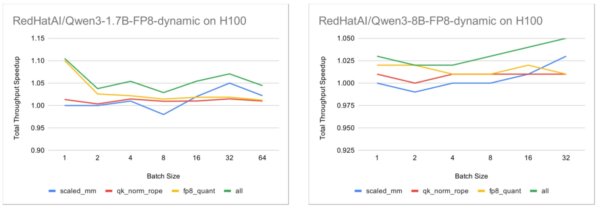
Fig. 1: Total throughput speedup on H100 with per-token activation quantization enabled, using the default vLLM setup as the baseline.
For the 1.7B model, the results show approximately 1.05x end-to-end throughput improvement on H100 when all Helion kernel groups are enabled. For the 8B model, the improvement is most pronounced around batch size 32, which aligns with the kernel-level observations where Helion scaled_mm achieves its strongest performance around num_tokens = 32.
We also evaluated speculative decoding scenarios where the effective decode-phase num_tokens naturally falls into this performance sweet spot.
Using:
- RedHatAI/Qwen3-8B-speculator.eagle3
- RedHatAI/Qwen3-32B-speculator.eagle3
we observed up to approximately 1.09x end-to-end throughput improvement when all Helion kernels were enabled.
| Batch Size | Model | # Speculative Tokens (per-pos acc rate) | Helion TTFT
(mean, ms) |
Default TTFT
(mean, ms) |
TTFT Speedup | Helion TPOT
(mean, ms) |
Default TPOT (mean, ms) | TPOT Speedup | Helion Total Throughput
(tok/s) |
Default Total Throughput
(tok/s) |
Total Throughput Speedup |
| 16 | Qwen3-8B | 1 (47%) | 34.75 | 39.93 | 1.15x | 4.63 | 5.01 | 1.08x | 6,314.86 | 5817.23 | 1.09x |
| 16 | Qwen3-8B | 3 (35%, 25%, 15%) | 38.46 | 51.18 | 1.33x | 4.40 | 4.63 | 1.05x | 6,616.60 | 6261.1 | 1.06x |
| 8 | Qwen3-32B | 2 (24%, 10%) | 81.92 | 100.93 | 1.23x | 13.29 | 14.37 | 1.08x | 1,101.61 | 1018.32 | 1.08x |
| 8 | Qwen3-32B | 3 (24%, 10%, 4%) | 83.01 | 104.73 | 1.26x | 13.33 | 14.21 | 1.07x | 1,100.04 | 1030.51 | 1.07x |
Tab. 3: End-to-end benchmark results on H100 with per-token activation quantization and speculative decoding enabled. Acceptance rates for speculative tokens are reported in parentheses.
On NVIDIA B200, we enabled only the fp8_quant kernel group during end-to-end evaluation. The remaining kernel groups either:
- underperformed relative to the baseline (Triton limitation for Blackwell GEMMs)
- or showed inconsistent gains across traffic patterns.
Even with only the quantization-related kernels enabled, we still observed meaningful throughput improvements across all tested Qwen3 model sizes.
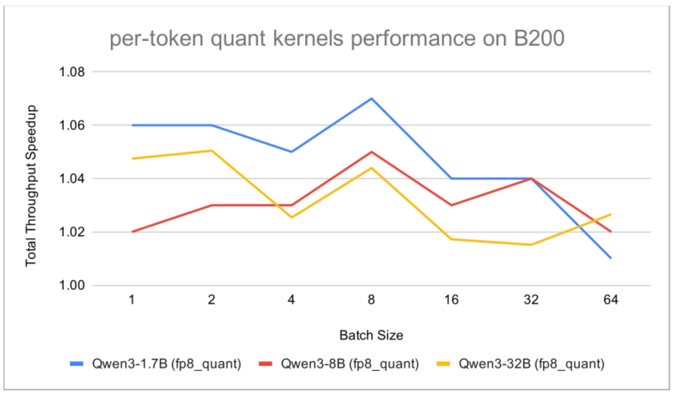
Fig. 2: Total throughput speedup on B200 with per-token activation quantization enabled, using the default vLLM setup as the baseline.
Dynamic per-group activation quantization
For per-group activation quantization, we used the following checkpoints:
- Qwen/Qwen3-1.7B-FP8
- Qwen/Qwen3-8B-FP8
- Qwen/Qwen3-32B-FP8
For per-group activation quantization, DeepGEMM is the default backend for blockwise FP8 GEMM on both H100 and B200. However, our current per-group Helion quantization kernels are not yet compatible with the UE8M0 quantization format required by DeepGEMM. Therefore, for this experiment, we forced vLLM to use CUTLASS as the linear backend.
This means the baseline in this section is not the default vLLM configuration. However, the comparison is still meaningful because we are able to use consistent CUTLASS kernels for the linear layer for all runs. As a result, the measured differences come from the non-GEMM kernels being evaluated, such as FP8 quantization and fused quantization kernels, rather than from changes in the linear backend.
The following figures show enabling only the small Helion kernels still produced approximately 1.05x end-to-end throughput improvement across all workloads.
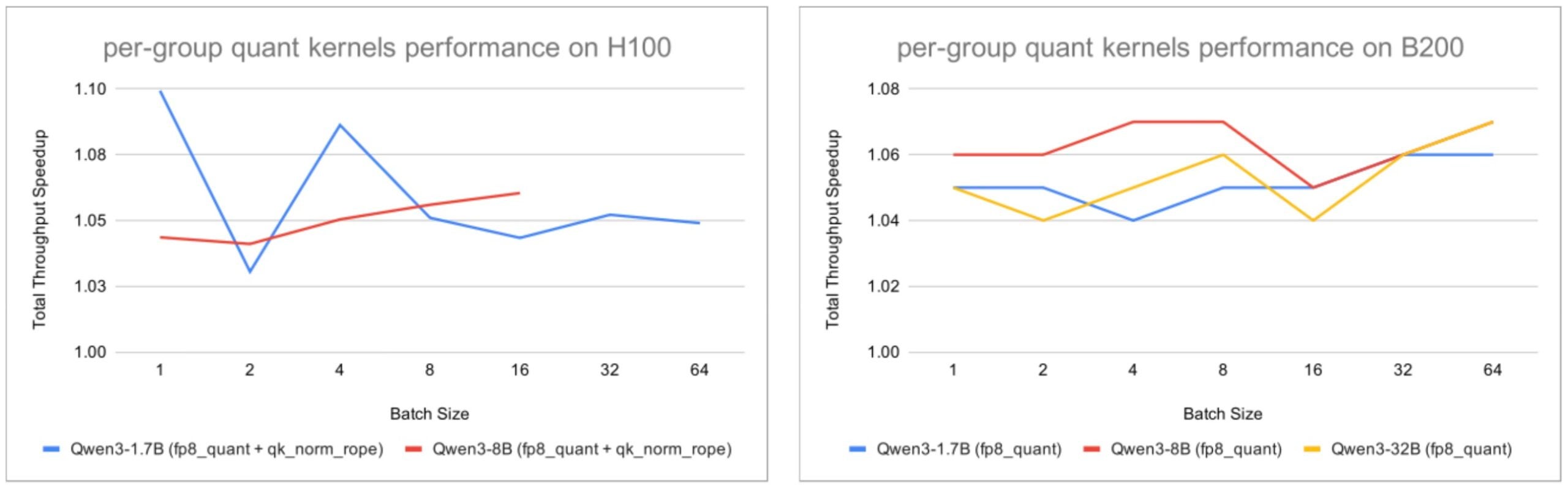
Fig. 3: Total throughput speedup on H100 and B200 with per-group activation quantization enabled, using the default vLLM setup with the linear layer backend replaced by CUTLASS as the baseline.
Resources
For reproducibility and further exploration, all Helion kernel implementations discussed in this post are linked in the corresponding GitHub issue. The same issue also includes the vLLM branches used in our experiments for reproducing the reported end-to-end benchmark results.
Caveats
During our experiments, the majority of engineering time was spent on kernel autotuning. For large kernels such as scaled_mm, running a full-effort autotuning sweep across all three model sizes, covering a total of 168 distinct input shapes, can take an entire day, as Helion automatically generates and benchmarks thousands of candidate kernel implementations for each shape. Initial research suggests that exhaustive per-shape autotuning and dispatching may not always be necessary, and that reducing the number of specialization buckets may achieve a better tradeoff between autotuning cost and runtime performance with minimal performance degradation. The Helion team is actively exploring additional techniques to further reduce tuning time, including search-space reduction strategies and LLM-guided autotuning approaches.
Another caveat is that Helion runtime dispatching itself introduces tens of microseconds of CPU overhead per kernel launch. For small kernels, this overhead can dominate the end-to-end latency. As a result, CUDA graph capture and replay are essential for achieving optimal performance with Helion kernels. The Helion team is actively reducing the dispatch latency without CudaGraph mode.
Conclusion
Helion provides a natural, PyTorch-syntax-centric approach for writing kernels in a tile-programming style. It significantly simplifies kernel development and reduces implementation effort. In our experiments, most kernels could be implemented and validated within a single day, demonstrating that Helion is a practical DSL for rapidly developing new kernels and exploring kernel fusion opportunities.
Combined with its powerful AOT autotuning capability, Helion demonstrated strong potential for achieving high performance. Our experiments show that Helion kernels deliver strong performance for many kernels and consistently outperform the default vLLM implementations in most cases. For GEMM kernels, there is still room for improvement to match or exceed CUTLASS performance, particularly on Blackwell GPUs, the teams are actively working to improve it by improving Triton code gen and introducing alternative backends like CuteDSL.
Acknowledgments
This work was supported by many contributors across the OCTO and vLLM teams at Red Hat, as well as the Helion team at Meta. In particular, we would like to thank our colleagues: Luka Govedič, Richard Zou and Will Feng for their feedback and support throughout this work.
Using Muon Optimizer with DeepSpeed
3 Jun 2026, 3:05 pmTL;DR
DeepSpeed now supports Muon Optimizer! Muon Optimizer has gained great momentum with significant adoption from frontier AI Labs. One of those AI Labs is Moonshot AI, which has adopted Muon Optimizer to train its Large Foundation Model like Kimi-K2-Thinking. This post dives into what Muon Optimizer is and how it performs on DeepSpeed.
What is Muon Optimizer?
Muon is an optimizer designed for hidden 2D weights of a neural network. It takes gradient of the weight, computes its momentum, and applies Newton-Schulz iterations to orthogonalize the momentum matrix, then uses this orthogonalized matrix to update the weight. Because Muon only maintains one momentum buffer (versus Adam’s two), it uses less memory for optimizer states.
The orthogonalization step is key to Muon’s convergence advantage in pretraining. In practice, gradient updates for 2D weights in transformers tend to have very high condition numbers — they are nearly low-rank, dominated by a few large singular directions. By orthogonalizing the momentum matrix, Muon equalizes all singular values, effectively amplifying rare but important update directions that would otherwise be overshadowed. This leads to better sample efficiency: in NanoGPT speedrunning benchmarks, Muon improved training speed by 35% over AdamW, and at 1.5B parameter scale it reached GPT-2 XL level performance approximately 25% faster than AdamW.
Unlike Adam optimizer that requires two momentum buffers for each parameter, Muon Optimizer only requires one momentum buffer. This means that for parameters using Muon Optimizer, we only need to allocate one buffer for momentum, which can save memory compared to Adam.
Muon is used by Keller Jordan’s mod of NanoGPT, Andrej Karpathy’s nanochat, and a variant of Muon (MuonClip) is also used by the production-level LLM Kimi-K2 from MoonShot. More recently, Zhipu AI’s GLM-5 (744B parameters) confirmed the use of Muon Optimizer in both GLM-4.5 and GLM-5 pretraining, along with a “Muon Split” technique that splits MLA up-projection matrices by attention head and orthogonalizes each head independently, addressing a performance gap between MLA and GQA when using Muon DeepSeek-V4 (1.6T parameters) also employs the Muon Optimizer for faster convergence and greater training stability.
Muon Optimizer support in DeepSpeed
One of the challenges of applying Muon optimizer to DeepSpeed is that previous optimizers (SGD, Adam) look at gradients as flattened buffers. Thus it is hard to swap in Muon Optimizer in the same place because the gradient buffers are already flattened. We move the Muon update to get_flat_partition function of stage 1 and 2 DeepSpeedZeroOptimizer in which per parameter gradients are still in unflattened stages, thus we can easily apply the Muon updates.
Muon Optimizer works on 2D weight matrices (attention and MLP weights). It applies Newton-Schulz orthogonalization to the momentum matrix, which requires the weight to be 2D. Non-2D parameters (embeddings, layer norms, biases, lm_head) fall back to AdamW. We apply a parse in model engine initializer to tag the model parameter with use_muon, if and only if the model parameter is 2D and belongs to hidden layers. When Muon Optimizer is used, any parameter tagged use_muon will use Muon Optimizer to update weight.
Note that Muon is a hybrid optimizer: it uses Muon updates only for 2D hidden weights and falls back to Adam for all other parameters (embeddings, layer norms, biases, lm_head). The DeepSpeed config supports separate learning rates via muon_lr(for Muon parameters) and adam_lr (for Adam parameters).
Running DeepSpeed finetune with Muon Optimizer
Deepspeed finetune demo is a demo to use different DeepSpeed training features and compare their performance in a single place. You can use it to test finetune LLM models with Muon Optimizer:
git clone https://github.com/delock/deepspeed_finetune_demo

cd deepspeed_finetune_demo
./finetune.sh z2_muon.json
Muon Optimizer Convergence Experiment Result
We tested Muon Optimizer by finetuning Moonlight-16B-A3B (a Mixture-of-Experts model with 16B total and 3B active parameters), and evaluated on code generation (MBPP/MBPP+), general knowledge (MMLU), and mathematical reasoning (GSM8K) benchmarks. Each benchmark uses its own domain-specific training set.
Training Configuration:
- Model: Moonlight-16B-A3B (MoE, 16B total / 3B active)
- Training datasets: sahil2801/CodeAlpaca-20k for MBPP/MBPP+, cais/mmlu (auxiliary_train, ~95k examples) for MMLU, meta-math/MetaMathQA (sample_rate=0.1, ~39.5k examples) for GSM8K
- ZeRO Stage 2, bf16, Expert Parallelism (autoep_size=4)
- Batch size: 16, gradient accumulation: 2, 4 GPUs
- 1 epoch, gradient clipping: 1.0
Evaluation Results
| Optimizer | Learning Rate | adam_lr (for Muon) | MBPP | MBPP+ | MMLU | GSM8K |
| baseline (pre-finetune) | — | — | 0.495 | 0.431 | 0.401 | 0.526 |
| AdamW | 2e-6 | — | 0.661 | 0.534 | 0.660 | 0.805 |
| Muon | 1e-4 | 2e-6 | 0.646 | 0.548 | 0.678 | 0.810 |
Muon outperforms AdamW on 3 out of 4 metrics: MBPP+ (0.548 vs 0.534, +1.4pp), MMLU (0.678 vs 0.660, +1.8pp), and GSM8K (0.810 vs 0.805, +0.5pp). On MBPP base tests, AdamW edges out Muon (0.661 vs 0.646, -1.5pp), though Muon achieves a higher score on the more rigorous MBPP+ with extra test cases (0.548 vs 0.534), suggesting better generalization.
Muon Optimizer Memory Savings
Muon Optimizer uses less memory for optimizer states than Adam, because it maintains one momentum buffer per parameter instead of two (first and second moment).
Memory Usage Comparison
Note that Muon is a hybrid optimizer: 2D hidden weights use Muon (1 buffer), while remaining parameters (embeddings, layer norms, lm_head) still use Adam (2 buffers). The actual memory savings depend on the fraction of parameters that are 2D hidden weights. For typical transformer models, approximately 90% of parameters are 2D hidden weights, so optimizer state memory is reduced by roughly 45%. However, because total GPU memory also includes model weights, gradients, and activations, the end-to-end memory reduction is smaller (see measured results below).
| Optimizer | State Buffers per Param | Memory per Parameter |
| Adam | 2 (m, v) | 8 bytes |
| Muon | 1 (momentum) | 4 bytes |
Measured GPU Memory: Qwen2.5-3B Fine-tuning
We measured peak GPU memory during fine-tuning Qwen2.5-3B on tatsu-lab/alpaca using the same 8xA100 (40GB) configuration described above (batch size 32, ZeRO Stage 2, bf16).
| Optimizer | Peak Memory per GPU | Savings vs AdamW |
| AdamW | 34.5 GiB | — |
| Muon | 31.4 GiB | 9% |
Muon reduces per-GPU memory by approximately 3 GiB (9%) compared to AdamW. The savings come entirely from optimizer states: Muon parameters store one momentum buffer (4 bytes) instead of Adam’s two (8 bytes). However, because optimizer states are only one component of total GPU memory (alongside model weights, gradients, and activations), the end-to-end reduction is modest. For larger models or tighter memory budgets, this 9% savings could make the difference between fitting a workload on-device versus requiring CPU offloading.
What’s Next
Muon is rapidly gaining traction in the community, and production-level adoption by Kimi-K2 (1T parameters) and GLM-5 (744B parameters) signals that it is a serious contender to replace Adam as the default optimizer for large-scale training. We are actively building out full Muon support in DeepSpeed, with a series of improvements already in flight:
- ZeRO Stage 2 support — merged
- ZeRO Stage 3 support — merged
- Gram-Schmidt based Newton-Schulz iteration — a faster orthogonalization kernel, in review
- CPU Offloading — in progress
- MuonClip — the variant used by Kimi-K2, planned
We welcome any thoughts, feedback and contributions related to Muon Optimizer support on DeepSpeed – please start an issue for discussion or submit a PR to DeepSpeed. Let’s make Muon rock solid and lightning fast in DeepSpeed!
How LinkedIn Uses PyTorch to Solve Extreme-Scale Optimization Problems
1 Jun 2026, 2:53 pm
TL;DR: This case study demonstrates how LinkedIn re-architected its distributed linear programming solver, DuaLip, by developing a GPU-accelerated PyTorch version to handle extreme-scale optimization challenges like web applications. This transition from a CPU-bound stack achieved order-of-magnitude speedups and efficient multi-GPU scaling while reducing engineering overhead.
Introduction
Modern internet platforms don’t just make predictions; they also make decisions. At companies like LinkedIn, these decisions power the intelligent behavior of large-scale web applications.
Behind the scenes, many of these systems reduce to a deceptively simple question:
Given millions (or billions) of options, what is the best set of actions to take under constraints?
This is where linear programming (LP) comes in as a foundational mathematical framework for optimizing an objective under constraints. At LinkedIn scale, these LPs can involve hundreds of millions of users and trillions of decision variables, with sparse but highly structured constraint matrices. Traditional LP solvers, such as simplex and interior-point methods, have historically been the workhorses of optimization. However, they rely on matrix factorizations or basis updates that become prohibitively expensive in both memory and computation at extreme scale. As a result, they often fail to handle modern web-scale problems efficiently.
The Business Challenge
Our goal was to optimize large-scale decision systems under competing objectives.
Examples include:
- Matching jobs to potential job seekers
- Balancing multiple business metrics in a ranking or recommendation system.
- Optimizing the volume of emails to be sent to users
These are inherently challenging optimization problems, where improving one metric (e.g., clicks) may hurt another (e.g., complaints). Formally, these problems are expressed as linear programs:
- Objective: maximize business value (e.g., engagement, revenue)
- Constraints: enforce limits (e.g., budget, fairness, frequency)
The key bottleneck is scalability: as the problem size grows, supporting fast, repeatable optimization in production requires implementations that are both memory- and time-efficient, while maintaining stability and solution quality.
In recent years, first-order methods have emerged as a practical alternative for solving such massive LPs. Unlike classical approaches, these methods rely only on gradient information and avoid expensive matrix factorizations, making their core operations dominated by matrix–vector multiplications. In particular, primal-dual formulations have proven especially effective: they recast the LP as a saddle-point problem and iteratively update primal and dual variables until convergence, often achieving sufficiently accurate solutions for production systems.
This line of work has led to a new generation of large-scale solvers, including systems like PDLP at Google and DuaLip at LinkedIn. DuaLip, in particular, is a distributed solver based on ridge-regularized dual ascent and first-order optimization. It exploits the decomposable structure of matching problems and uses accelerated gradient-based updates along with efficient projection operators to scale to extreme problem sizes.
While DuaLip demonstrates that first-order methods can handle web-scale LPs in production, its original implementation, built on a Scala/Spark stack, remains fundamentally CPU-bound. This limits its ability to fully leverage modern hardware accelerators. Additionally, its schema-bound, template-driven interface makes it difficult to extend to new problem formulations, slowing iteration for evolving use cases.
Motivated by these limitations, we re-architect the DuaLip solver stack in PyTorch with GPU acceleration, resulting in DuaLip-GPU as a modern, flexible, and scalable system for industrial-scale optimization.
How LinkedIn Uses PyTorch
To address these challenges, we propose DuaLip-PyTorch as a core execution engine for large-scale optimization—not just deep learning. The system is built around an operator-level array/tensor programming model (in the style of PyTorch’s define-by-run paradigm), rather than a task-level “call a solver” API.
Concretely, the hot path is expressed as an explicit dataflow over sparse matrix–vector operations and blockwise projections, orchestrated by a lightweight maximizer. This design boundary is intentional: it exposes the kernels that dominate runtime, enables flexible choices of sparse layouts and projection operators, and maps naturally to GPU execution—all without requiring changes to the core optimization loop.
Solving AI Challenges with PyTorch
PyTorch provides native GPU acceleration, flexible tensor abstractions for both sparse and dense computation, and efficient matrix-vector operations for gradient computation. Together, these capabilities allow large-scale LP solving to look structurally similar to neural network training, but with optimization-specific primitives. At LinkedIn, these features helped address three major systems and optimization challenges.
First, extreme-scale LPs containing billions to trillions of variables were implemented using sparse tensor operations and batched projection kernels, enabling efficient execution on GPUs.
Second, distributed optimization was achieved by partitioning variables across GPUs while replicating and synchronizing dual variables through collective communication patterns such as all-reduce and broadcast, allowing near-linear scaling across devices.
Third, convergence speed was improved through a combination of row normalization and scaling for better conditioning, regularization continuation strategies, and scalable first-order optimization methods including AGD and FISTA-style variants. These improvements significantly reduce solve time while maintaining accuracy.
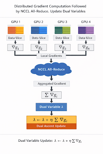
Figure 1. High-level architecture of Dualip-Pytorch
The Benefits of Using PyTorch
Using PyTorch allowed LinkedIn to:
- Achieve order-of-magnitude speedups over CPU-based systems
- Scale efficiently from single GPU to multi-GPU systems
- Support flexible, extensible LP formulations
- Reduce engineering overhead for new optimization problems
- Bridge ML and optimization into a unified stack
Most importantly, it enabled production-grade optimization at previously infeasible scales by restructuring the solver around GPU-efficient sparse linear algebra.
The dominant computation in DuaLip-Pytorch consists of repeated sparse matrix–vector multiplications and projection updates, which map naturally to high-throughput GPU execution. By expressing these operations as batched tensor kernels in PyTorch and distributing them across multiple GPUs with synchronous collective communication, the system achieved significantly lower per-iteration solve time compared to the original CPU-based implementation.
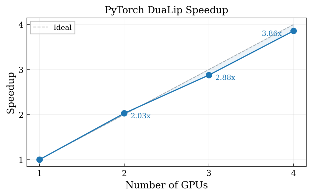
Figure 2. Speed up curve against the number of GPUs compared to the ideal (linear line). All GPUs are located on one node.
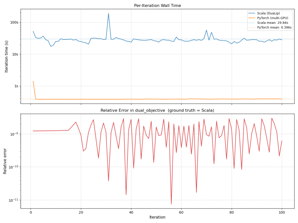
Figure 3. Scala-Pytorch comparison in terms of speed and relative error. Pytorch solver (8 GPUs) exhibits significant gain (75 times faster) in per-iteration wall clock time.
Learn More
For more information:
- DuaLip-GPU Technical Report: https://arxiv.org/abs/2603.04621
- Open-source implementation: https://github.com/linkedin/DuaLip
Why Is PyTorch Compile So Fast: Kernel Fusion
27 May 2026, 7:09 pmWhen you use PyTorch’s compiler, your model runs faster, up to 10x faster. But what’s actually happening? Without compilation, the GPU runs a kernel, a function on the GPU, for each torch operation in your code. This creates two big slowdowns: the time spent moving data in memory, and the overhead of starting each new kernel. Every time the GPU launches a kernel, it pays an overhead cost, and every intermediate result means writing to and reading from memory.
This is where fusion comes in. PyTorch’s Inductor compiler automatically groups dependent operations together into single, efficient Triton kernels. This keeps data in faster memory close to the register and cuts down on kernel overhead. In this article, we’ll look at a concrete example of fusion, and then outline topics for further reading. You’ll see exactly how torch.compile transforms your PyTorch operations into optimized GPU code.
To get the most out of this article, you should have basic familiarity with PyTorch and a general understanding of GPU programming concepts.
What is Vertical Fusion?
Think of vertical fusion as a way to “link” steps, so the output of one goes straight into the next. It’s called “vertical” because if you picture the computation graph, these operations stack vertically – each one depends on the result of the previous step.
This is the most common fusion pattern in deep learning because neural networks are chains of operations: normalization, then linear layers, then activation functions, and so on. The big win is eliminating intermediate results – those temporary tensors never need to be written to or read from global memory. They stay in fast registers where the GPU can reach them more quickly.
Let’s dive into an example of vertical fusion, namely pointwise fusion.
Pointwise Fusion Example
Pointwise operations are simple math kernels that work on each element: addition, multiplication, activation functions, and more. Let’s look at a pattern you might see in a neural network layer:
Pointwise PyTorch Example
Unfused: Three Separate kernels
Without fusion, Inductor creates three separate Triton kernels. Don’t worry if the Triton syntax looks intimidating. The important part isn’t memorizing the syntax, but understanding the pattern: each kernel loads data, does one operation, and writes the result.
Kernel 1: Multiply
For succinctness, we include just the signatures of the next kernels as they are nearly identical, see our Git Repository for the full source code.
Kernel 2: Add
Kernel 3: Sigmoid
Across the three kernels you’re performing eight memory operations: reading inputs twice for multiply, reading multiply’s result and the bias for add, reading add’s result for sigmoid, and writing all three results. That’s a lot of memory traffic.
Fused: One Kernel
With fusion, torch.compile creates a single kernel:
Kernel 4: Fused
Notice the difference: we load all inputs once, do all three operations in a row, and store only the final result. The intermediate values (tmp2 and tmp4) stay in registers – the fastest memory on the GPU. They never touch the slower global memory.
Benefits
- Kernel launches: 3 reduced to 1
- Intermediate buffers: 2 eliminated (multiply result and add result)
- Memory bandwidth: Reading 5 full tensors and writing 3 full tensors (8 memory operations) reduced to reading 3 tensors and writing 1 (4 memory operations) – a 50% reduction in memory traffic
Other Fusion Types
Pointwise fusion is just one type of vertical fusion. Inductor uses other forms of vertical fusion to keep your GPU efficient:
Reduction Fusion: Combines reducing operations like max, mean, or sum, with the operations that happen before and after them. This is critical for operations like batch normalization.
GEMM + Epilogue Fusion: Attaches simple math to the end of heavy matrix calculations. Instead of doing a matrix multiply, writing the result to memory, then reading it back to add bias and apply ReLU, the bias and activation happen right after the multiply in the same kernel.
Prologue Fusion: The opposite of epilogue – preprocessing happens as data loads. For instance, normalizing input before matrix multiplication can happen on-the-fly as the data comes in.
In addition to vertical fusion, the most prominent type of fusion, Inductor also uses horizontal fusion.
Horizontal Fusion: Runs multiple independent operations on the same input at once. For example, computing both sin(x) and cos(x) in a single kernel, loading x only once instead of twice.
Get Started: See Fusion in Your Own Code
Let’s walk through a complete example using a reduction pattern.
Step 1: Create a Simple Reduction Example
Create a file called fusion_example.py:
Step 2: View the Generated Code
Run your script with the TORCH_LOGS environment variable to see what Inductor generated:
This outputs the generated Triton kernels to your terminal. Look for a kernel named something like triton_per_fused_add_mul_sum_0. The per prefix means “per-reduction” kernel, and the name tells you that add, mul, and sum were all fused together.
Conclusion
Fusion is one of the most important optimizations that torch.compile does. By linking dependent operations into single kernels, it cuts down memory traffic and kernel overhead – often the main slowdowns in GPU work.
Try accelerating your own code with torch compile. No need to change your implementation, just add a torch compiler decorator and let the compiler do the work.
Learn more: PyTorch documentation at pytorch.org/docs/stable/torch.compiler.html has complete guides on compilation and optimization strategies. Reference our Git Repository for the full source code.
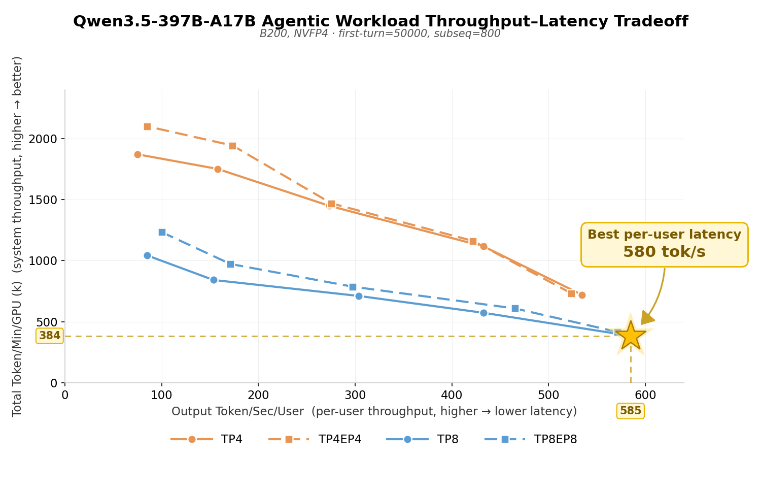
Up to 580tps! New Speed Record of Qwen3.5-397B-A17B on GPU for Agentic Workloads with TokenSpeed
27 May 2026, 3:39 pmTL;DR: The TokenSpeed inference engine achieved a record-breaking 580 tps running the Qwen3.5-397B-A17B model on GPUs. This extreme performance for agentic workloads is driven by systematic elimination of memory copies, advanced kernel fusions, and fully overlapped CPU-GPU execution-keeping the GPU saturated at all times. On the functionality side, TokenSpeed also supports hybrid prefix caching and unified Prefill-Decode state transfers to handle complex agentic serving scenarios.
1. Introduction
The Qwen open-source models represent a highly capable family of large language models designed for broad accessibility and flexible deployment. They feature a comprehensive matrix of open-source versions with varying parameter sizes, catering to diverse scenarios from resource-efficient edge devices to complex cloud environments. Trained on extensive, high-quality corpora, these models demonstrate exceptional proficiency in natural language understanding, advanced logical reasoning, full-stack coding, and ultra-long context processing. Furthermore, with built-in support for autonomous agent planning, multi-step task execution, and tool calling, the Qwen open-source lineup empowers developers and researchers worldwide to efficiently build, customize, and deploy powerful AI applications.
Qwen3.5 models, the flagship of Qwen open-source lineup, push the boundaries further by adopting a hybrid attention mechanism that interleaves standard full attention layers with linear attention layers based on the Gated Delta Network (GDN). Unlike traditional pure-Transformer architectures, this hybrid design maintains strong modeling capabilities while significantly reducing computational complexity for long-sequence inference.
TokenSpeed is a high-performance, open-source LLM inference engine released by the LightSeek Foundation under the MIT license, purpose-built for agentic workloads. It aims to deliver “speed-of-light” performance comparable to TensorRT-LLM while maintaining the developer-friendly usability of vLLM. Built from the ground up with a native SPMD architecture and static compilation, it significantly accelerates the execution of complex multi-step agent tasks, empowering developers to efficiently deploy ultra-fast, production-grade AI applications.
This post presents the complete design, implementation, and optimization of Qwen3.5 models in the TokenSpeed inference framework, covering runtime architecture design (PD disaggregation, prefix caching, scheduler), key performance optimizations, and performance benchmarks.
2. Runtime Designs and Features
Qwen3.5 uses a hybrid architecture: most layers are GDN (linear attention with per-layer conv_state and temporal_state), with every N-th layer being standard full attention with a conventional KV cache. TokenSpeed provides full GDN-aware support across prefix caching, scheduling, and prefill-decode disaggregation, enabling efficient serving of the entire hybrid stack.
2.1 GDN/Mamba prefix cache
Prefix cache is critical to agentic workloads, where multi-turn tool-calling sequences frequently share long contexts and conversation histories. TokenSpeed’s prefix cache is split across two layers. C++ owns the logical cache: radix-tree matching, page IDs, eviction, and Mamba slot lifetime. Python owns the physical tensors: GPU KV pages, Mamba conv_state / ssm_state, stream ordering, copy-on-write, zeroing, and snapshot copies.
For the normal KV cache, a prefix hit means reusing cached page IDs. For Mamba, that is not enough. A reusable prefix must also carry the recurrent state at the same prefix boundary. TokenSpeed solves this by attaching a MambaSlot to the same radix-tree node that represents the cached KV prefix.
Slot Lifecycle
Each active Mamba request may hold two slot types:
workingslot: mutable state used by the current forward step.checkpointslot: snapshot destination that can later be published to the prefix tree.
The scheduler allocates these slots in C++, but Python writes the actual tensor contents.
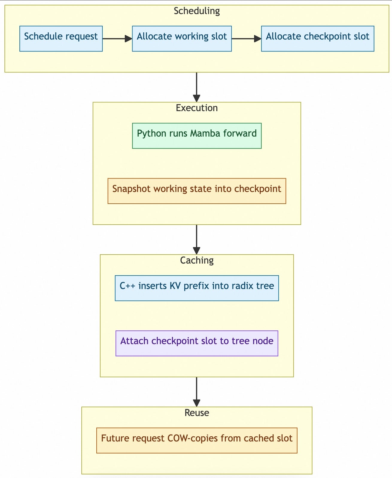
A checkpoint slot becomes reusable only after two things are true: Python has populated it with a clean state, and C++ has attached it to a block-aligned radix-tree node.
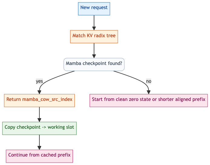
Prefix Match and Copy-on-Write
When a future request matches the tree, HybridPrefixCache first performs the normal KV prefix match, then finds the nearest Mamba checkpoint node. If such a node exists, the scheduler returns mamba_cow_src_index.
Python then copies that cached checkpoint into the request’s private working slot before running forward. The cached tree slot is not mutated; only the request’s working slot changes.
Keeping Checkpoints Clean
The main correctness risk is stale data in reused slots: MambaChunkAllocator hands out integer slot IDs without clearing GPU memory. TokenSpeed prevents stale state through runtime rules.
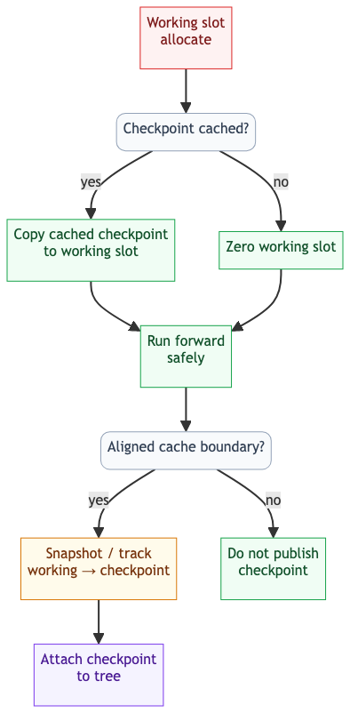
Concretely, a newly allocated working slot is guaranteed safe in exactly two ways: it either receives a copy-on-write copy from a known-clean checkpoint, or Python explicitly zeroes it before use. Checkpoints are published only at aligned boundaries, so the tree never advertises arbitrary intermediate state as reusable prefix state.
Chunked Prefill Under Overlap Scheduling
Chunked prefill introduces a subtlety in overlap mode: the CPU may schedule the next chunk before it commits the previous chunk’s output. The checkpoint is still safe because of CUDA stream ordering.
The previous chunk’s Mamba forward writes the checkpoint on execution_stream. At the start of the next loop iteration, the default stream waits for execution_stream. Only after that does C++ insert the previous chunk into the tree and detach its checkpoint slot. The next chunk then gets a fresh checkpoint slot.
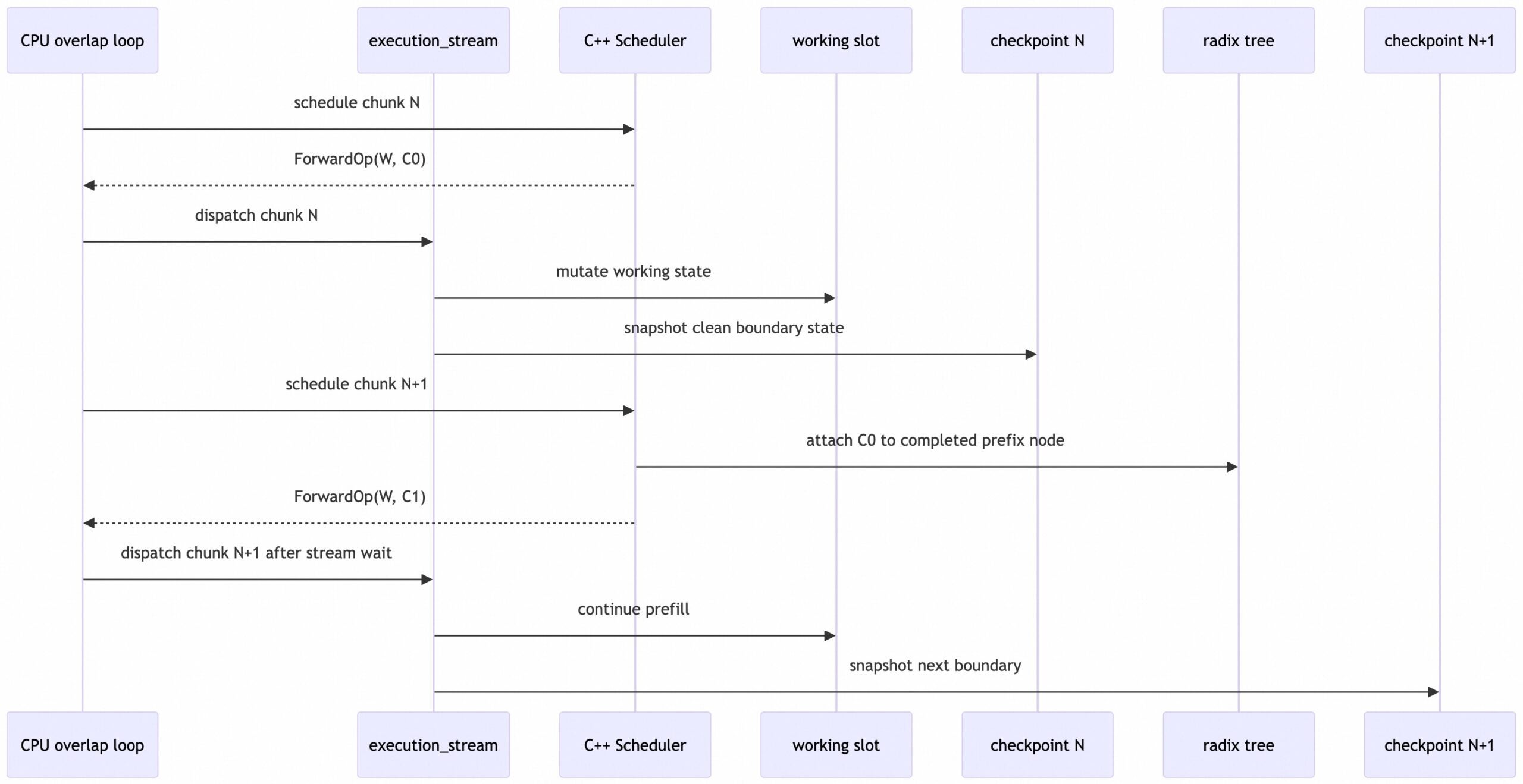
The key invariant is:
C++ may publish the checkpoint slot ID during overlap scheduling, but any later GPU consumer is ordered after the previous chunk’s snapshot write, and the published slot is no longer reused as the next checkpoint destination.
Decode Overlap
Decode has a different hazard: the next decode may mutate the same working slot before the CPU has committed the previous result. TokenSpeed handles this by snapshotting block-aligned decode states before dispatching the next decode.
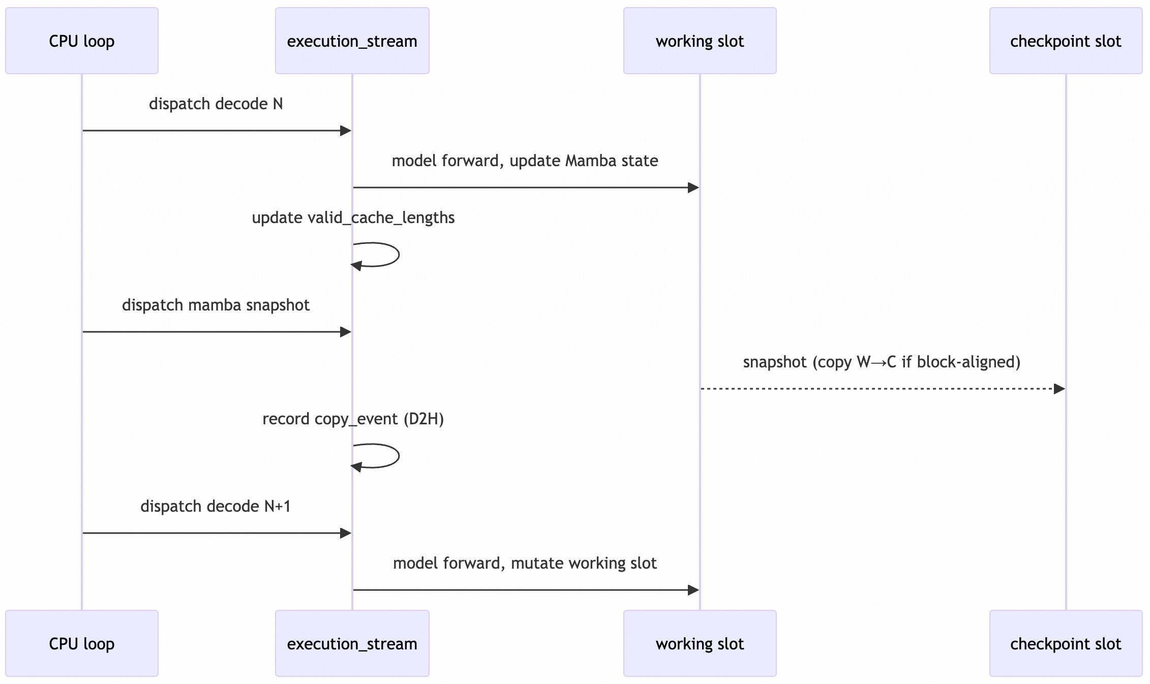
This preserves the clean state before the working slot advances.
Summary
TokenSpeed’s Mamba prefix cache is safe because it treats Mamba state as a tree-owned checkpoint, not as an incidental side effect of a request. C++ controls when a slot becomes part of the prefix tree. Python controls when the tensor contents are copied, zeroed, and snapshotted. Together they maintain one central invariant: every Mamba slot reachable from the prefix tree contains a clean, aligned state for the prefix represented by that tree node.
2.2 Scheduler
The hybrid architecture places unique requirements on the scheduler: it must simultaneously manage KV Cache (full attention layers) and Mamba State (linear attention layers) as two separate resource pools.
Mamba State and Hybrid Model Management
TokenSpeed’s scheduler implements the following key mechanisms:
- Dual Resource Pool Management: Each request holds both KV Cache block indices and Mamba Pool slot indices (
mamba_pool_indices), with the scheduler managing allocation and release for both. - State Lifecycle:
- On request arrival: allocate mamba_pool slot
- During prefill: populate initial state (or load from prefix cache)
- During decode: update state in-place each step
- On completion or preemption: release slot
- Speculative Decoding Support: The scheduler maintains intermediate state cache (
spec_cache) storing Conv/SSM state snapshots for each speculative step, enabling rollback upon verification failure. - Layer-Level Routing:
HybridLinearAttnBackendroutes forward calls to the appropriate backend (full attention or linear attention) based onlayer_id, with separate metadata initialization for each backend type.
2.3 GDN PD
2.3.1 The Challenge
For hybrid models, mamba layers maintain state tensors beyond conventional key-value pairs. These states must be transferred from prefill nodes to decode nodes alongside KV caches, requiring correct layer-wise alignment between full-attention and Mamba layers.
2.3.2 What We Built
We introduce end-to-end Mamba cache support for PD disaggregation, including:
1. Unified State Transfer: Two Worlds, One Wire
The core insight is that Mamba states, despite their different semantics, can be transferred using the same RDMA machinery as KV caches — as long as the system knows how to address them.
We designed a dual-tensor pool on each node: one pool holds convolutional states (the short-term memory of causal convolutions), the other holds recurrent SSM states (the long-term compressed history). Both are pre-allocated as contiguous GPU memory, with each request owning exactly one slot per layer. At registration time, the prefill and decode nodes exchange buffer descriptors — base addresses, per-slot sizes, and a mapping from each physical buffer to its corresponding global layer ID.
When transfer begins, the system maps each request’s slot indices into physical byte offsets, groups contiguous slots into scatter-gather blocks, and issues them as bulk RDMA writes. From the network’s perspective, Mamba states are just another set of memory regions — no serialization, no intermediate staging. The key difference is the addressing: KV caches are indexed by page tables, while Mamba states are indexed by flat slot IDs assigned by the scheduler.
2. Cross-Layer Scheduling: A Unified Heartbeat
The most subtle piece of the puzzle is when to transfer each layer’s state.
In layerwise transfer mode, the prefill node doesn’t wait for the entire forward pass to finish before starting data movement. Instead, it begins shipping data as soon as each layer group completes — overlapping computation with communication. But for a hybrid model, this means the transfer thread must track progress across both attention layers and Mamba layers as if they were one continuous pipeline.
We introduced a unified step counter that ticks once after every layer’s forward pass — regardless of type. The transfer thread watches this counter and, for each layer window, sends whichever data belongs to that window: KV pages for full-attention layers, state slots for Mamba layers. The model’s layer-type pattern becomes invisible to the transfer logic — it simply asks “which buffers map to layers 4 through 7?” and sends them all once the counter reaches 7.
On the decode side, the mirror of this mechanism is a layer-done barrier: the model forward can begin executing layer 0 before layer 15’s state has arrived. Each layer’s computation calls into the state pool, which blocks only if that specific layer hasn’t been loaded yet. This allows decode to overlap network reception with early-layer execution, hiding transfer latency behind useful work.
3. PD-Aware Token Lifecycle: The Three-Phase Handshake
The final piece connects state transfer to the token generation lifecycle. In a disaggregated system, the prefill node doesn’t just produce states — it also produces the first output token. The decode node needs both before it can begin generation.
We designed a three-phase handshake:
- Transfer completes: All KV pages and Mamba states for the final layer group are shipped. But the transfer thread doesn’t declare success yet — it holds at a barrier, waiting for the forward pass to finish.
- Token produced: The prefill forward completes and emits the first output token. The event loop records this token and signals the waiting transfer thread.
- Status delivered: The transfer thread sends a lightweight status message (carrying the bootstrap token) to the decode endpoint via a side channel. Only when the decode node receives both the bulk state data and this token does it emit a “remote prefill done” event to its scheduler.
This protocol ensures an invariant: the decode node never begins generation with incomplete state, and never wastes a step re-deriving the first token. The Mamba states, the KV cache, and the bootstrap token arrive as a logically atomic unit — even though they travel through different paths and at different times.
3. Performance Optimizations
3.1 Mamba State Update Optimization
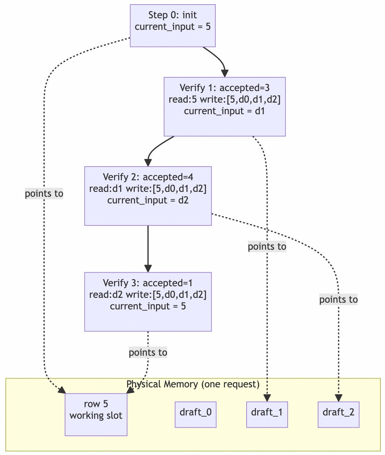
Eliminating Mamba State Copies with Index Indirection
In speculative decoding with Mamba-style linear attention, the target-verify phase traditionally carries a hidden memory cost. After the draft model produces speculative tokens, the base model runs forward to validate them. Because each draft token advances the Mamba state by one step, the engine needs to preserve intermediate states for every speculative position, then recover the correct one based on how many tokens were accepted.
The previous pipeline handled this with a dedicated intermediate state cache: the kernel wrote per-step Mamba states into a side buffer during verify, and a post-verify fused_mamba_state_scatter_with_mask kernel copied the state at the accepted position back into the scheduler-owned working slot. The scatter itself was a full tensor copy across num_layers × state_dim —not free, and executed on every decoding step.
The Core Idea: Move Pointers, Not Data
Instead of buffering intermediate states in a separate cache and scattering the accepted one afterward, we let the kernel write each step’s output directly to a dedicated physical row, then simply remember which row holds the canonical state.
The state buffer is extended with a draft region appended after the scheduler-allocated base slots; each request owns a private slice of draft rows indexed by its req_pool_index. A lightweight table current_input_indices records, for each request, which physical row currently holds its canonical Mamba state.
During target-verify:
- Input redirection: The kernel reads its initial state from the row recorded in
current_input_indices(which may be a working slot, a COW-forked slot, or a draft row from a previous step). No data movement happens here—only an index lookup. - Output routing: A per-request
output_state_indicestensor tells the kernel exactly where to write each step’s output: slot 0 is the working row, slot 1..N are the request-private draft rows. The kernel writes directly into these pre-assigned locations, eliminating the intermediate cache entirely. - Post-verify bookkeeping: Once the accepted length is known, we simply update
current_input_indices [req]to point at the draft row corresponding to the last accepted token. This is an O(1) integer write, not an O(L·D) tensor copy.
3.2 Runtime Optimization
3.2.1 Overlap Is All You Need
Following common practice in modern inference engines, TokenSpeed employs CUDA multi-stream parallelism to overlap non-sequential operations. By executing independent workloads concurrently across multiple streams, TokenSpeed effectively reduces scheduling overhead and improves end-to-end latency.
Shared Expert and Routed Expert Overlap
Qwen3.5 MoE layers contain shared experts and routed experts. Shared experts process all tokens while routed experts only handle TopK-selected tokens. The two are naturally parallelizable and are implemented via the StreamFork class for stream forking and synchronization:
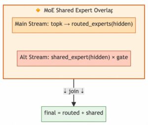
- Main stream executes TopK routing, expert dispatch, and MoE GEMM
- Auxiliary stream concurrently executes shared expert forward (gate_up → SiLU → down) and sigmoid gating
- Both streams synchronize via events before combining results
This overlap hides shared expert computation latency, reducing single MoE layer time in production deployments.
GDN Input Projection Dual-Stream Optimization
The GatedDeltaNet layer’s input projection contains two independent linear layers (in_proj_qkvz and in_proj_ba), also executed in parallel across streams:
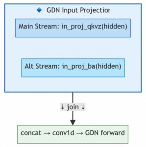
This optimization is only activated during CUDA Graph capture, where the smaller in_proj_ba projection is fully hidden behind the larger in_proj_qkvz on the alternate stream.
3.2.2 The More You Fuse, The Less Latency You Get
Gemma AllReduce Fusion
GemmaRMSNorm uses x * (1 + weight) instead of standard RMSNorm’s x * weight, which previously prevented use of TRT-LLM’s fused AllReduce + Residual + RMSNorm kernel.
TokenSpeed pre-computes gemma_weight = weight + 1.0 and passes it as the gamma parameter to the standard fused kernel — to enable GemmaRMSNorm communication fusion. After fusion, AllReduce + residual addition + RMSNorm per layer is merged from three separate kernel launches into one:
This fusion covers all Qwen3.5 decoder layers and auto-enables on SM90+ single-node TP deployments.
Fused QK-RMSNorm + Partial RoPE + Gate Split in Attention
In the original attention path, after the QKV GEMM projection, 5 separate kernels are launched sequentially to normalize, rotate, and split the Q/K/gate vectors:
| Step | Operation | Read from HBM | Write to HBM |
|---|---|---|---|
| 1 | Q RMSNorm | q | q_normed |
| 2 | K RMSNorm | k | k_normed |
| 3 | Q RoPE | q_normed | q_rotated |
| 4 | K RoPE | k_normed | k_rotated |
| 5 | Gate split + contiguous copy | q_gate | gate |
Each intermediate tensor (q_normed, k_normed, etc.) is written to global memory only to be immediately read by the next kernel — pure bandwidth waste. fused_qk_rmsnorm_rope_gate replaces all 5 launches with a single Triton kernel. All intermediate values stay in registers.
Fused Gate-Sigmoid-Mul-Add in MoE Shared Expert
In the MoE block, the shared expert output is gated before merging with routed expert output. The original code path launches 5 separate kernels for what is conceptually one expression:
| Step | Kernel | Note |
|---|---|---|
| 1 | Elementwise multiply | h[i] * w[i] — per-element products |
| 2 | Reduce | Sum partial products → 1 scalar per token |
| 3 | Sigmoid | σ(gate_val)— elementwise on the scalar |
| 4 | Multiply | σ(gate_val) * shared_output— broadcast scalar × full vector |
| 5 | Add | final_hidden_states += scaled |
The key inefficiency: gate_valis a scalar per token, yet the unfused path materializes both the per-element products and the reduced scalar to HBM between launches. The intermediate scaled tensor (full [num_tokens, hidden_dim]) is also written and immediately re-read. fused_gate_sigmoid_mul_addcomputes the full expression final += σ(x·w) * shared in one Triton kernel, in-place. The dot-product reduction, sigmoid, broadcast multiply, and accumulate all happen within a single thread block per token — intermediates never leave registers.
3.2.3 Death by a Thousand Syncs
TokenSpeed’s decode loop captures the core forward pass — target model, sampler, and draft model — into a single CUDA graph. Once captured, thousands of GPU kernels replay with one launch, eliminating per-kernel dispatch overhead entirely.
But CUDA graphs are static by design. Between graph replays, the runtime must still perform dynamic work on the host: preparing inputs, resolving scheduling indices, updating Mamba state pointers after speculative verification, and coordinating transfer state. These “gaps” between graphs are where CPU overhead hides — and where a careless .item() or an unnecessary D2H copy can stall the entire pipeline.
TokenSpeed treats this inter-graph CPU overhead as a first-class optimization target: keep the host out of the critical path, even outside the graph.
Eliminating Device-to-Host Round-Trips
The most insidious sync pattern is the “innocent query” — reading a single scalar from GPU to make a branching decision on the host. TokenSpeed replaces these with pre-computed worst-case bounds known at initialization, or captures CPU-side maximums before H2D transfer so both the GPU tensor and its bound are available simultaneously. For speculative decoding state management, boundary detection and slot selection use GPU-side sentinel values — downstream kernels skip invalid entries via bounds checks rather than CPU-side filtering. The entire decision tree stays on device.
Compile-Fused Index Arithmetic
Runtime scheduling in hybrid models involves heavy index manipulation: computing slot mappings, draft-token layouts, and pointer updates after verification. In eager PyTorch, each step becomes a separate kernel launch with intermediates written to HBM. TokenSpeed annotates these routines with torch.compile, allowing Inductor to fuse 10–14 individual launches into one or two elementwise kernels where all values flow through registers. The GPU stays busy, and the CPU submits one launch instead of fourteen.
Asynchronous Everything
H2D transfers use pinned memory with non-blocking copies throughout. The transfer system polls pinned-host counters instead of calling synchronize(), and layer-wise loading uses event-based barriers that wake only the specific layer that needs data. The CPU prepares the next batch while the current one is still in flight.
The cumulative effect: TokenSpeed’s decode loop maintains near-zero CPU overhead — the host thread spends its time submitting work, not waiting for results.
3.3 FA4 Support
Flash Attention 4 (FA4) is the next-generation attention kernel targeting NVIDIA Blackwell architecture. Qwen3.5 uses head_dim=256 by default, placing substantial demands on attention compute backends — a configuration that not all kernels support efficiently out of the box.
Support for FA4 with head_dim=256 has been contributed and merged into the upstream community repository. In TokenSpeed, native FA4 support for Qwen3.5 is currently under active development and will be available in an upcoming release, further unlocking the full compute potential of Blackwell GPUs for Qwen3.5 inference.
4. Benchmark
Taking Qwen3.5-397B-A17B as a representative example, we present a systematic performance evaluation of Qwen3.5 models on NVIDIA Blackwell GPUs. We would like to thank the EvalScope team for providing the benchmarking tool; all performance results reported below are obtained using EvalScope Benchmark.
Test Environment: All benchmarks were conducted using the TokenSpeed latest Docker image (lightseekorg/tokenspeed-runner:latest), based on the recent version. The benchmark scripts and reproduction instructions are available at TokenSpeed’s GitHub repository.
4.1 Basic Benchmark
We use fixed input/output lengths and measure decode throughput (output token/s). We evaluated performance across varying batch sizes under different parallelism configurations (TP/EP). Two primary test configurations were used:
- Config 1: Attn TP + MoE TP
- Config 2: Attn TP + MoE EP
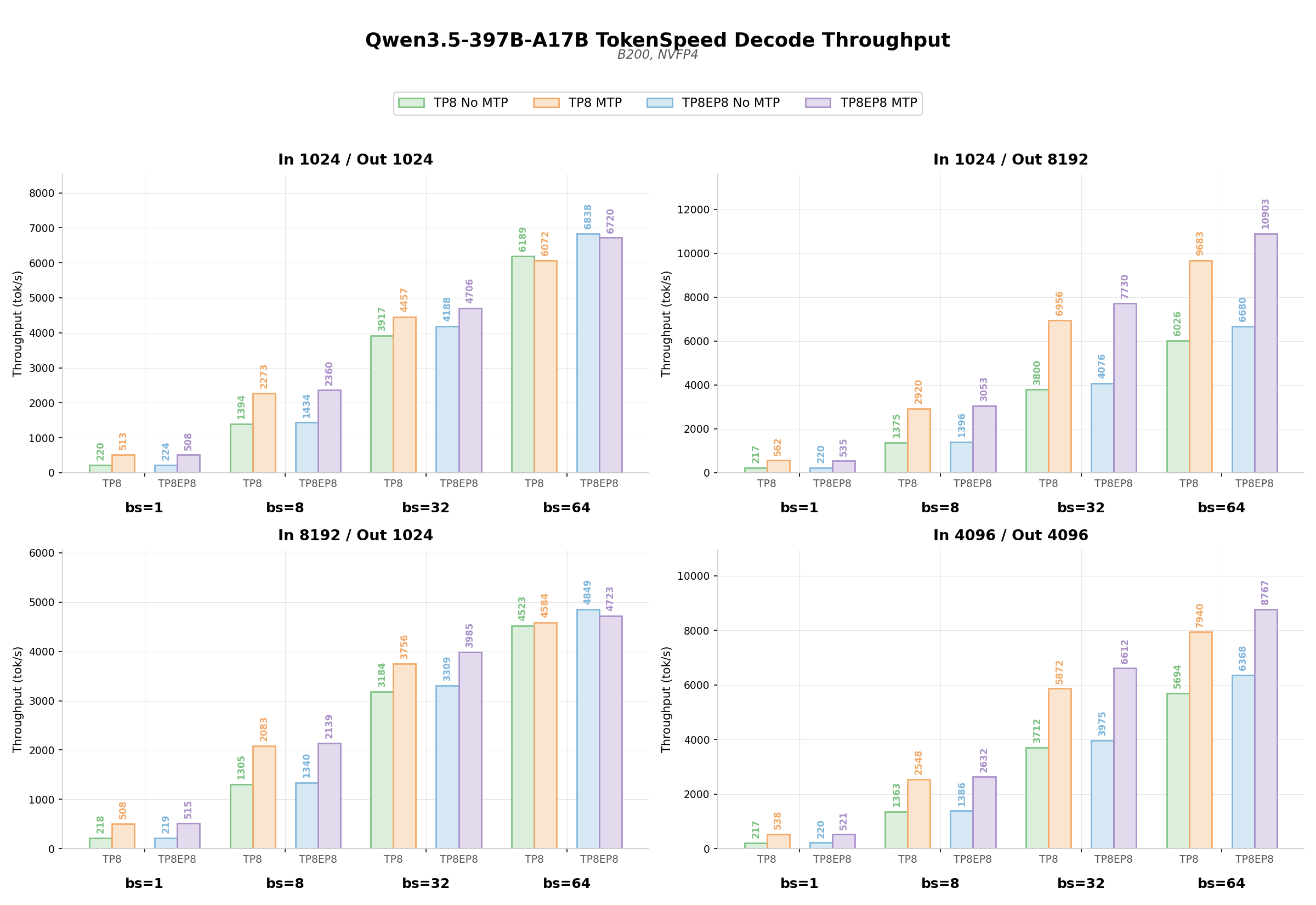
We benchmarked Qwen3.5-397B-A17B-NVFP4 decode throughput on B200 with MTP enabled and disabled.
Across all input/output length configurations on Attn TP8 + MoE TP8 / Attn TP8 + MoE EP8, MTP delivers +100%~+159% throughput gains at bs=1, where latency is the primary bottleneck. At higher concurrency, the gain is strongly correlated with output length: long-output workloads (e.g., output length >4096) sustain substantial speedups of +38%~+90% at bs=32 / 64, while short-output workloads (e.g., 1024 tokens) at bs=64 see gains diminish to near-zero or turn slightly negative, as speculation overhead begins to outweigh acceptance benefits when decoding is already throughput-bound.
4.2 Agentic Workload Benchmark
The rapid proliferation of Agent applications — encompassing tool call histories and multi-turn dialogue context — has fundamentally reshaped the characteristics of production workloads. To reflect real-world agent behavior, we use the Agentic Workload test suite that simulates realistic agent call patterns (50K first-turn context, 800 tokens appended per subsequent turn, 10-15 turns total).
On B200 with NVFP4, TokenSpeed delivers exceptional single-user throughput for Qwen3.5-397B-A17B under agentic workloads. All four parallelism configurations — TP4, TP4EP4, TP8, and TP8EP8 — sustain 500+ tok/s at bs=1, with TP8 achieving a peak of ~580 tok/s.
At concurrent=16, the TP4 family scales to ~2K tok/min/GPU system throughput while the TP8 family reaches ~1K tok/min/GPU. Pure-TP and TP+EP configurations within the same GPU count exhibit comparable throughput-latency tradeoffs, giving users deployment flexibility without sacrificing performance. Notably, the multi-turn agentic workload achieves an average KV cache hit rate exceeding 90%, significantly reducing prefill overhead and contributing to the overall throughput gains.
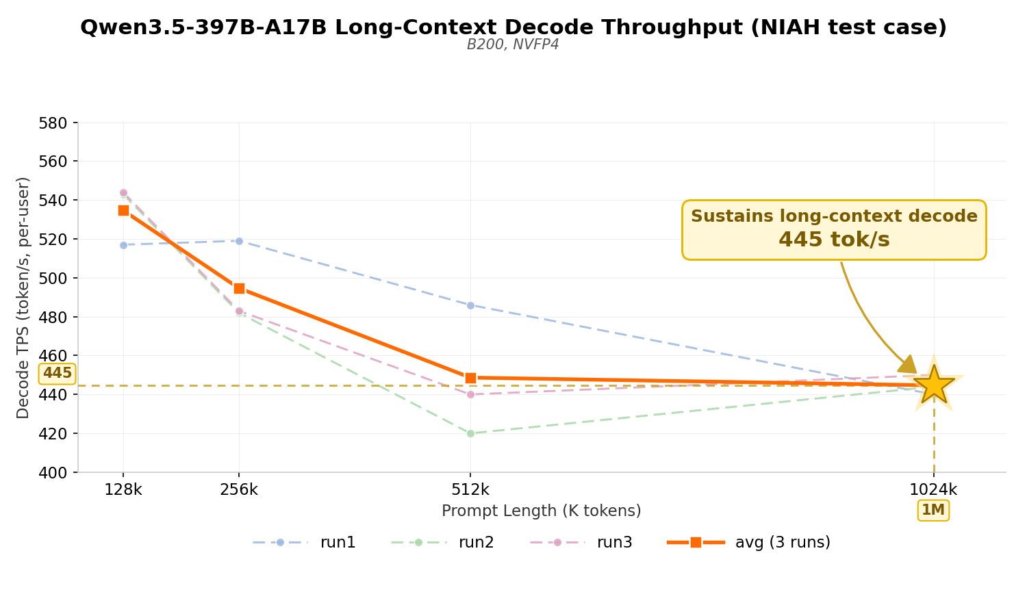
4.3 Up-to-1M Long Context Benchmark
Long-context handling is another key challenge in Agent workloads. While Prefix Cache can hit large amounts of repeated prefixes across multi-turn conversations and significantly reduce Prefill overhead, the Decode stage still has to read and attend to the full historical KV at every step, which the cache cannot bypass — the longer the context, the higher the per-step Decode memory-access cost.
Based on the NIAH (Needle-in-a-Haystack) 1M sample, we sliced four prompt lengths — 128K / 256K / 512K / 1M — for evaluation. On Qwen3.5-397B-A17B, decode throughput remains at ~530 tok/s/user within 128K, ~495 at 256K, and ~445 at 1M (measured on TP8), giving an end-to-end degradation of only ~16% from 128K to 1M — long-context throughput decay is kept well under control.
5. Conclusion
Through the optimizations and architectural designs described above, TokenSpeed delivers outstanding performance for the Qwen3.5 models — particularly in agentic workloads, achieving ultra-low latency generation and high inference throughput. TokenSpeed will continue to push the boundaries of Qwen inference optimization, pursuing ever more extreme performance at every level of the stack.
We invite you to follow the TokenSpeed project and experience speed-of-light inference throughput for yourself. A complete installation guide is available on GitHub, making it straightforward to deploy and benchmark on supported hardware. We also warmly welcome performance-oriented pull requests from the community — every contribution helps the Qwen model series run faster and smarter.
6. Acknowledgements
This work was made possible through close collaboration across the open-source ecosystem. We would like to thank Alibaba Tongyi Team, NVIDIA DevTech, the Mooncake Team, and the LightSeek Foundation for their engineering collaboration and implementation support. We also thank NVIDIA and Verda for providing Blackwell GPU infrastructure and compute support.
Alibaba Cloud Joins the PyTorch Foundation as a Platinum Member
27 May 2026, 1:00 am
The PyTorch Foundation, a community-driven hub for open source AI under the Linux Foundation, is announcing today that Alibaba Cloud has joined as a Platinum member.
Alibaba Cloud is a global leader in full-stack artificial intelligence services, offering state-of-the-art intelligent capabilities and a worldwide AI cloud computing network, providing developer-friendly AI services across the globe. Qwen, the family of large language and multimodal AI models developed by Alibaba, has become one of the most influential and widely adopted open-weight model series since its debut in 2023, earning strong recognition from the global developer communities.
“We believe the future of AI is built on open, production-proven infrastructure — and PyTorch sits at the heart of that future. Joining the PyTorch Foundation is a natural step given our years of running PyTorch at scale across heterogeneous hardware on Alibaba Cloud. We look forward to working alongside the PyTorch Foundation to raise the bar for AI infrastructure and help developers build the next generation of models with confidence,” said Dr. Feifei Li, Chief Technology Officer of Alibaba Cloud.
As a dedicated member, Alibaba Cloud aims to drive the PyTorch ecosystem forward in two ways: by delivering a seamless, out-of-the-box experience across all hardware and by contributing our production-hardened engineering expertise, including AI compiler optimization, multi-chip compatibility, and large-scale stability practices, to the upstream community.
Alibaba Cloud also maintains its own PyTorch distribution that closely tracks the upstream, delivering high performance and stability across large-scale AI workloads — both internally across Alibaba Group and externally for cloud customers.
Alibaba Cloud’s commitment to heterogeneous hardware support has been a key driver of its deep engagement with PyTorch. It ensures consistent framework quality and compatibility across a wide range of accelerators — providing developers with a unified experience regardless of the underlying hardware.
On the engineering scale, PyTorch at Alibaba powers large-cluster training and inference workloads internally. Externally, it underpins key ecosystem projects including SGLang, vLLM, PAI-TurboX, and TorchEasyRec, serving Alibaba Cloud customers across production-scale LLM training and inference, autonomous driving, embodied AI, and recommendation systems.
“We are delighted to welcome Alibaba Cloud to the PyTorch Foundation as a Platinum member,” said PyTorch Foundation Executive Director, Mark Collier. “Alibaba’s recent launch of new AI accelerators for the agentic era that are powered by PyTorch and consistent support for open source will be invaluable as the PyTorch Foundation continues to grow into a multi-project home that sustains the entire AI lifecycle from training and optimization to production-grade inference.”
As a platinum member, Alibaba Cloud is granted one seat to the PyTorch Foundation Governing Board. The Board sets policy through our bylaws, mission and vision statements, describing the overarching scope of foundation initiatives, technical vision, and direction.
We’re happy to welcome Junhua Wang, Vice President of Alibaba Cloud, to our board. Junhua Wang is responsible for Alibaba Cloud’s big data platform and machine learning platform, supporting the large-scale data storage, compute, analytics and machine learning needs within Alibaba Group while powering Alibaba Cloud’s enterprise customers from various industries. Alibaba Cloud big data platform and machine learning platform is dedicated to building the core foundation of Agentic AI. By focusing on four key pillars—models, AI infrastructure, data infrastructure, and end-to-end development tools—it provides robust technical support for the deployment of top-tier large language models and complex Agent systems.
We’re also pleased to welcome Tao Ma, Principal Engineer at Alibaba Cloud, to the PyTorch Foundation’s Technical Advisory Council (TAC). Tao Ma leads a team responsible for the design and development of Alibaba Cloud’s foundational software. The team’s primary work encompasses underlying operating system technologies for cloud computing, compiler technologies, and foundational technologies related to AI inference and training optimization. Their goal is to build a world-leading underlying AI infrastructure platform that supports the rapid development of cloud and AI.
To learn more about how your organization can join the PyTorch Foundation, visit our website.
About PyTorch Foundation
The PyTorch Foundation is a community-driven hub supporting the open source PyTorch framework and a broader portfolio of innovative open source AI projects, including DeepSpeed, Helion, PyTorch, Ray, Safetensors, and vLLM. Hosted by the Linux Foundation, the PyTorch Foundation provides a vendor-neutral, trusted home for collaboration across the AI lifecycle—from model training and inference, to domain-specific applications. Through open governance, strategic support, and a global contributor community, the PyTorch Foundation empowers developers, researchers, and enterprises to build and deploy AI at scale. Learn more at https://pytorch.org/foundation.
TLX Block Attention: A Warp-Specialized Blackwell Kernel for Fixed-Block Sparse Self-Attention
26 May 2026, 1:26 pmCode available at: https://github.com/facebookresearch/ads_model_kernel_library
In this post, we present the design of TLX Block Attention — a Triton kernel targeting NVIDIA Blackwell GPUs that exploits compile-time knowledge of a block-diagonal attention pattern to eliminate entire categories of algorithmic overhead present in general-purpose attention implementations. On NVIDIA B200 GPUs, the kernel achieves a ~1.85× forward and ~2.50× backward speedup over Flash Attention v2, and a ~3.5× speedup for the combined attention-and-rotary backward pass when rotary embeddings are fused into the attention epilogue.
This work is built on TLX (Triton Language Extensions) — a set of low-level extensions to the Triton compiler that expose hardware-native control over warp specialization, asynchronous tensor core operations, and memory hierarchy management on NVIDIA Blackwell GPUs. TLX bridges the gap between Triton’s high-level Python productivity and the fine-grained hardware control traditionally requiring raw CUDA or CUTLASS. For more on TLX, see the triton-ext repository
───────────────────────────────────────
1. Introduction
Self-attention is a mechanism that lets a model weigh how relevant each element in a sequence is to every other element — essentially asking “which parts of this input should inform my understanding of each other part?” It’s the core building block of Transformer architectures and is what allows these models to capture rich, context-dependent relationships in data. A good intuition might be: how do one’s past decisions inform present and future ones?
Block-diagonal self-attention — where the sequence is partitioned into fixed-size groups that attend only within themselves — is a widely-used pattern in recommendation and feature-interaction models (BlockBERT, Qiu et al., EMNLP 2020) [1]. In our ads ranking stack, production workloads typically run batch sizes of 1152 with sequences up to ~4k tokens, head dimensions of 64 or 128, and ~70% sparsity in the attention structure with increasing sequence lengths. As these models grow deeper and wider, attention cost becomes the dominant bottleneck.
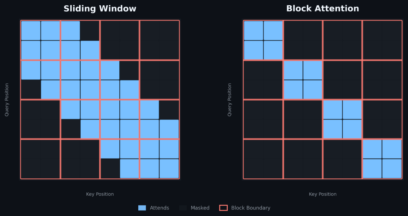 Today these workloads run on general-purpose kernels like Flash Attention v2 with block masking or sliding window. FlexAttention (FA4) [7] supports block-sparse patterns but operates at a minimum tile size of 256 — incompatible with the 64-token blocks these models require. Flash Attention v2 with block masking remains the strongest available baseline at this tile size, but leaves significant performance on the table. Flash Attention’s tiled iteration, online softmax correction, logsumexp bookkeeping, and auxiliary kernel launches are essential for arbitrary-length causal attention — but pure overhead when the pattern is block-diagonal and known at compile time.
The central thesis of this work: when you know your attention pattern at compile time, you can build something much faster. We exploit the fixed constraint that every Q tile attends to exactly one K/V tile, propagating this knowledge through the entire algorithm to collapse multi-iteration accumulators into single GEMMs, eliminate correction stages, and remove auxiliary kernel launches.
───────────────────────────────────────
2. Why Block Attention?
2.1 The Fixed-Block Constraint and Its Cascade of Simplifications
Standard Flash Attention [2] handles sequences of arbitrary length by iterating a Q tile over multiple K/V tiles, maintaining running statistics (row-wise max and log-sum-exp) and applying a correction factor at each step to preserve numerical stability:
Listing 1: Standard Flash Attention inner loop showing multi-tile iteration and online softmax correction.
# Flash Attention inner loop (standard)
for k_tile in K_tiles:
    S = Q @ k_tile.T                   # partial scores
    m_new = max(m_old, rowmax(S))
    alpha = exp(m_old - m_new)         # correction factor
    O = alpha * O + exp(S - m_new) @ v_tile
    l = alpha * l + rowsum(exp(S - m_new))
O = O / l                              # final normalization
# Store L = m + log(l) to HBM for backward
This is correct and elegant for arbitrary sequences. But for block-diagonal attention with a fixed 64-token block size, the entire Q-tile-over-K-tiles loop is reduced to a single iteration. Every Q tile and its corresponding K/V tile are the same tile. That single constraint cascades through the algorithm:
- No multi-tile iteration. The score matrix S = Q · Kᵀ ∈ ℝ^{64×64} is complete after one GEMM. There is no loop to maintain state across.
- No online softmax correction. Since there is only one tile, the row-wise max and sum computed over S are globally correct immediately. The correction factor α = exp(m_old − m_new) is identically 1 and can be dropped entirely.
- No logsumexp (L) storage. Flash Attention stores the per-row log-sum-exp L to HBM so that the backward pass can recompute softmax. With a single tile, the backward pass can recompute P = softmax(S) directly from Q, K, V without any auxiliary tensor — eliminating an entire HBM write and read per forward/backward pair.
- No Di preprocessing kernel. The standard Flash Attention backward launches a separate kernel to compute Di = rowsum(dO ⊙ O) before the main backward pass. In TLX Block Attention, Di is computed inline within the dP/dS backward stage, eliminating a kernel launch and its associated memory traffic.
- No output accumulation with rescaling. With a single tile, the output O = P · V is a fresh result from a single GEMM, not an accumulation of multiple rescaled partial results. This enables
use_acc=Falseon all async_dot calls — telling the tensor core hardware that the TMEM accumulator need not be preserved across calls, allowing it to be freely reused.
Listing 2: use_acc=False signals to the hardware that no cross-tile accumulation is needed, enabling TMEM reuse.
# From the kernel: use_acc=False signals no accumulation needed
tlx.async_dot(
    q_tile[buff_idx],
    k_tile_T,
    TMEMqk[tmem_idx],
    use_acc=False,           # Fresh result — no accumulation
    mBarriers=[qk_SMEM_free[buff_idx], qk_TMEM_full[tmem_idx]],
)
2.2 Comparison with Standard Flash Attention
The following table summarizes the algorithmic differences:
| Aspect | Standard Flash Attention | TLX Block Attention |
| K tiles per Q tile | Many (full sequence) | Exactly 1 (same block) |
| Score matrix | Multiple tiles accumulated | Single [64, 64] — complete |
| Logsumexp L tensor | Stored to HBM for backward | Not needed |
| Running max/sum | Maintained across tiles | Computed once, consumed in-register |
| Correction factor α | Required every iteration | Not needed (dropped) |
| Output accumulation | Incremental with rescaling | Single P·V GEMM |
| use_acc mode | True (accumulate across tiles) | False (fresh result) |
| Di preprocessing | Separate kernel launch | Computed inline |
Table 1: Algorithmic differences between standard Flash Attention and TLX Block Attention.
These are not micro-optimizations — they represent the elimination of entire algorithmic stages. The backward pass in particular benefits substantially: the absence of a stored L tensor removes a round-trip through HBM per batch × heads × sequence, and inline Di computation removes a kernel launch with its associated driver overhead and memory bandwidth.
───────────────────────────────────────
3. Kernel Architecture: A Warp-Specialized Pipeline
3.1 TLX
We chose Triton as the authoring framework because it provides a Python-native, tile-oriented programming model that maps naturally to the warp-specialized pipeline structure described below — while avoiding the boilerplate of raw CUDA or CUTLASS and remaining portable across compiler evolution. Triton’s TLX (Triton Language Extensions) further expose Blackwell-specific primitives like async_dot, local_trans, and explicit TMEM/SMEM barrier management at a level of abstraction that balances hardware control with developer productivity. In our experience, TLX delivers performance on par with (and often exceeding) lower-level alternatives while enabling significantly faster iteration due to its Python-native simplicity.
Specifically, this kernel relies on several TLX primitives that go beyond base Triton: tlx.async_dot for issuing warp-specialized tcgen05 MMA operations with explicit accumulator control; tlx.async_descriptor_load for TMA-driven SMEM fills; tlx.local_trans for TMEM-to-register transfers; and the mBarrier synchronization model that coordinates the producer-consumer pipeline across warp groups. These extensions are available in the triton-ext repository.
3.2 Warp Specialization
TLX Block Attention uses warp specialization [8] — different warps within the same CTA are permanently assigned to different hardware units and execute different code paths throughout the kernel’s lifetime. This contrasts with the traditional CUDA model where all warps execute the same code and diverge only through conditionals.
| Stage | Warps | Registers | Hardware Unit | Role |
| Load | 1 | 48 | TMA engine | async_descriptor_load for Q, K, V |
| QK MMA | 1 | 48 | tcgen05 tensor cores | async_dot(Q, Kᵀ) → TMEMqk |
| Softmax | 4 | 120 | CUDA cores + SFU | mask / scale / exp2 / normalize → P to SMEM |
| PV MMA | 1 | 48 | tcgen05 tensor cores | async_dot(P, V) → TMEMpv |
| Epilogue | 8 | 200 | CUDA cores + L2 + TMA engine | TMEM → registers → BF16 → SMEM → TMAl store |
| Total | 15 | — | — | 480 threads per CTA |
Table 2: Forward pipeline stage configuration. Register allocations are deliberately asymmetric — hardware-accelerated stages receive minimal registers; CUDA core stages receive the most.
Fig. 1 — Forward pipeline warp timeline (conceptual, one iteration):

Time →
Load     [─ TMA Q,K ─][─ TMA V ─]
QK MMA         [── async_dot Q·Kᵀ ──]
Softmax                  [── exp2/normalize → P ──]
PV MMA                            [── async_dot P·V ──]
Epilogue                                   [── local_load → BF16 → store ──]
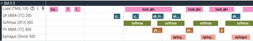
Each stage’s output signals a barrier that unblocks the next stage, creating a producer-consumer pipeline across hardware units. While the Epilogue warp writes tile i to global memory, the MMA warps are computing tile i+1, and the Load warp is fetching tile i+2 via TMA — three tiles in flight simultaneously.
3.3 The Roofline Context
At BLOCK_D=64, HEAD_DIM=128, arithmetic intensity is ~33 FLOP/byte — well below the B200’s ridge point of ~281 FLOP/byte [4]. The kernel is memory-bandwidth bound by design. This is why latency hiding via TMA and minimizing unnecessary memory traffic (the eliminated L tensor, the fused rotary) are the dominant optimization levers.
3.4 Buffer Management
To keep hardware units continuously busy, the kernel uses triple-buffered SMEM (3 slots) and double-buffered TMEM (2 slots), consuming ~169 KB of the 256 KB SMEM budget. With three SMEM slots, the Load warp can prefetch tile i+2 while the MMA warp processes tile i+1 and the Epilogue warp drains tile i. The backward kernel drops to double-buffered SMEM (~162 KB) to accommodate additional gradient tiles within the same 256 KB budget.
───────────────────────────────────────
4. The Backward Pass: Gradients Without the Logsumexp Tensor
In standard Flash Attention, the backward pass requires the forward pass to save the logsumexp tensor (L) to High Bandwidth Memory (HBM). This tensor is necessary to reconstruct the attention probabilities (P) during the backward pass. Furthermore, standard attention requires a separate preprocessing kernel to compute Δᵢ (row-wise sum of dO ⊙ out).
Because block-diagonal attention computes the entire 64×64 score matrix in a single tile, we can bypass both requirements completely. The backward kernel does not read any logsumexp tensor, nor does it require a separate preprocessing step. Instead, it fully recomputes S = Q · Kᵀ and P = softmax(S) inline — a cheap operation when the tile fits in a single pass.
This cascade of simplifications allows us to build a fully fused, 7-stage warp-specialized backward pipeline:
| Stage | Warps | Registers | Hardware Unit | Role |
| Load | 1 | 48 | TMA engine | Loads Q, K, V, dO (+ sin/cos for rotary) |
| QK MMA | 1 | 48 | tcgen05 tensor cores | Recomputes S = Q · Kᵀ |
| Softmax/P | 4 | 120 | CUDA cores + SFU | Recomputes P = softmax(S) |
| dV MMA | 1 | 48 | tcgen05 tensor cores | dV = Pᵀ · dO |
| dP/dS | 4 | 120 | TC + CUDA cores | dP = dO · Vᵀ, Δᵢ, dS |
| dQ/dK MMA | 1 | 48 | tcgen05 tensor cores | dQ = dS · K, dK = dSᵀ · Q |
| Epilogue | 8 | 200 | CUDA cores + L2 + TMA engine | Stores dQ, dK, dV (+ fused rotary) |
| Total | 20 | — | — | 640 threads per CTA |
Table 4: 7-stage backward pipeline configuration.
The backward pass is inherently more complex than the forward pass. It requires 20 warps (640 threads per CTA) to balance the intense computational requirements. Most notably, it fully saturates the 256 KB Tensor Memory on the SM. The five distinct TMEM buffers — TMEMqk, TMEMdv, TMEMdp, TMEMdq, and TMEMdk — collectively hit 100% TMEM utilization. To accommodate this, the backward kernel drops from triple-buffered SMEM in the forward pass to double-buffered SMEM (~162 KB / 256 KB, 63%), while keeping double-buffered TMEM.
───────────────────────────────────────
5. Scheduling for Variable-Length Sequences
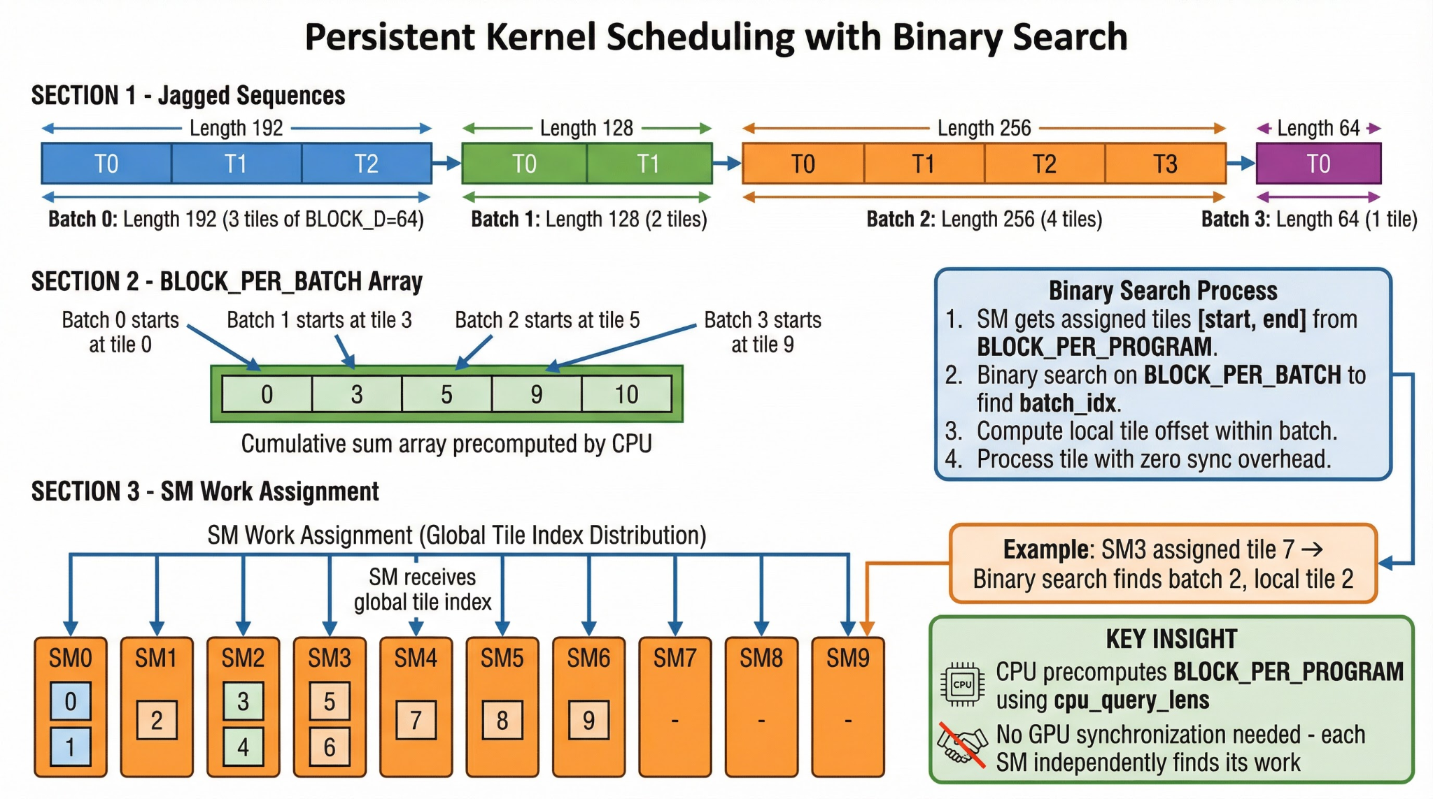 Real-world recommendation and feature interaction models do not process neatly uniform sequence lengths. Instead, traffic is dominated by jagged, variable-length sequences packed into a single flattened buffer. Naively mapping one CTA per sequence would leave SMs idle when short sequences finish early while others process long sequences — a severe workload imbalance.
To maximize SM occupancy, the kernel launches min(NUM_SMS, total_blocks) persistent programs — exactly one persistent thread block per SM. Workload is balanced across two precomputed arrays:
- BLOCK_PER_BATCH: A prefix-sum of the number of 64-token tiles per sequence.
- BLOCK_PER_PROGRAM: The balanced tile ranges assigned to each SM — computed using closed-form divmod arithmetic rather than cumulative sums.
To eliminate GPU synchronization overhead, when CPU-side offset tensors are available (cpu_offsets), all scalar scheduling arithmetic (tile counts, divmod, prefix sums) is computed on the CPU before the kernel launches — zero GPU sync points.
Inside the kernel, each SM must determine which sequence (batch index) a given global tile index belongs to. This uses a branchless binary search that executes in exactly 32 iterations (sufficient for any reasonable batch size) with zero thread synchronization.
───────────────────────────────────────
6. Fused Rotary Backward: Higher Precision at Higher Speed
For self attention layers, self attention is preceded by projection + sinusoidals [6]. In the backward pass this becomes attention backward -> sinusoidals which conventionally happen with 2 different kernel launches.
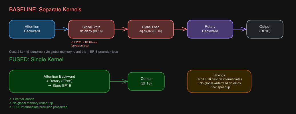 6.1 Baseline: Two-Kernel Backward Pass
The conventional backward pass requires two separate kernel launches:
- Attention Backward Kernel — accumulates dQ, dK, dV in FP32 via tensor cores, then truncates to BF16 on store to global memory.
- Rotary Backward Kernel — reloads the BF16 gradients from global memory, applies the rotary conjugate R(−θ), and stores the final BF16 result.
This separation has three costs:
| Problem | Impact |
| Precision loss | FP32 gradients are truncated to BF16 before the rotary transform — then truncated again on final store. Two quantization points, each injecting ~0.4% relative error (BF16 has only 7 mantissa bits). Downstream projection GEMMs amplify the accumulated error. |
| Memory bandwidth waste | dQ, dK, dV are written then immediately re-read — a full round-trip on a [total_seq_len, 1152] tensor (head_dim=128, 3 KV heads). With sequence lengths in the millions, this traffic is substantial. |
| Kernel launch overhead | Two separate dispatches where one suffices. |
6.2 Fused Approach
The attention backward kernel already dedicates a single warp group to the gradient store epilogue. We take advantage of this by injecting the rotary conjugate into that epilogue, while gradients are still in FP32 registers:
- Tensor cores store dQ, dK, dV in FP32 (TMEM).
- Load FP32 values into registers.
- Apply R(−θ) in full FP32 precision — a lightweight sin/cos load + element-wise multiply.
- Cast to BF16 and issue a single global store.
The per-step comparison:
| Aspect | Baseline (Separate) | Fused Kernel |
| Attention backward computation | FP32 | FP32 |
| Intermediate storage | BF16 → global memory | FP32 registers |
| Rotary sin/cos operations | BF16 | FP32 |
| BF16 quantization points | 2 | 1 (final store only) |
| Global memory round-trips | 2 | 0 |
| Kernel launches | 2 | 1 |
Fused rotary conjugate in the backward epilogue. The interleave operation applies R(−θ) to paired [cos, sin] components while still in FP32.
# Apply rotary conjugate to dV (neg_sin handles the conjugate)
dv0, dv1 = dvLocal.reshape(BLOCK_D, HALF_DIM, 2).split()
dvLocal = tl.interleave(
    dv0 * cos_local - dv1 * neg_sin,
    dv1 * cos_local + dv0 * neg_sin,
)
───────────────────────────────────────
7. Performance Results
All benchmarks were conducted on NVIDIA B200 GPUs (x86 cpu) with BF16 precision. The primary configuration uses B=1152 sequences, HEAD_DIM=128, H=4 heads, max_seq_len=2000, and sparsity=0.7 – discrete uniform (representative of production traffic distributions).
7.1 Kernel-Level Speedup
| Pass | Flash Attention v2 with block attention (ms) | TLX Block Attention (ms) | Speedup |
| Forward | 1.81 | 0.98 | 1.85× |
| Backward | 5.89 | 2.36 | 2.50× |
| Total | 7.70 | 3.33 | 2.31× |
Table 5: Kernel-level performance comparison (B=1152, D=128, H=4, BF16, B200, max_seq_len=2000, sparsity=0.7).
The backward speedup (2.50×) is larger than the forward speedup (1.85×) primarily because the backward pass benefits from two independent simplifications: (1) eliminated logsumexp storage and Di preprocessing, and (2) inline P recomputation that avoids the L-tensor HBM round-trip that standard Flash Attention backward requires.
7.2 Scaling Across Workloads
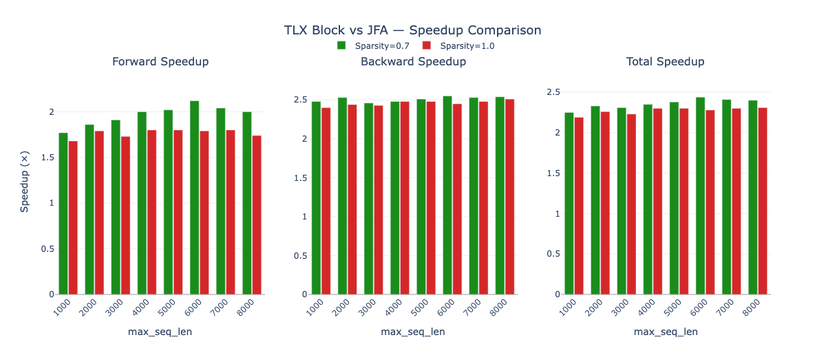
Table 6: Scaling performance across sequence lengths and sparsity ratios. Speedups are consistent regardless of distribution shape (batch=1152, for >7000 batch=768). Kernel speed up over flash attention v2 (jfa).
7.3 Fused Rotary Backward
The impact of fusing rotary backward into the attention epilogue is particularly striking:
| Configuration | Time (ms) |
| Attention backward (standalone) | 1.556 |
| Rotary backward (standalone) | 4.880 |
| Unfused total | 6.436 |
| Fused attention_rotary backward | 1.819 |
| Speedup | 3.54× |
Table 7: Fused vs. unfused rotary backward timing breakdown. The standalone rotary kernel dominates the unfused total. seq_len=1735537, heads=3, head_dim=128, batch=1152.
The standalone rotary backward is more than 3× more expensive than the attention backward itself — it is purely memory-bandwidth bound, reading and writing [M, D] tensors with no meaningful compute. Fusing it into the attention epilogue amortizes this bandwidth cost over the existing TMEM → register pipeline, reducing the combined operation from 6.436 ms to 1.819 ms.
End-to-end, integrating this kernel into self-attention layers results in a +30.6% Model FLOPs Utilization (MFU) gain on those layers.
7.4 Numerical Accuracy
Fusing the rotary backward into the FP32 epilogue also yields measurable accuracy improvements. Comparing against a high-precision PyTorch reference, TLX Block Attention reduces the maximum gradient error in the query gradients (dQ) by over 2×:
| Metric | Flash Attention v2 | TLX Block Attention | More Accurate |
| Max dQ diff | 0.2559 | 0.1201 | TLX |
| Max dK diff | 0.1689 | 0.1689 | Tie |
| Max dV diff | 0.0112 | 0.0112 | Tie |
| Avg dQ diff | 0.000309 | 0.000220 | TLX |
Table 8: Gradient numerical accuracy against a PyTorch reference implementation. TLX Block Attention reduces max dQ error by 53% due to the single-quantization-point fused rotary path.
dQ benefits most because the query gradient (dQ = dS · K) flows through the fused rotary conjugate with 1 quantization point instead of 2. dK also passes through the rotary conjugate (RoPE rotates both Q and K), but its maximum absolute error happens to be dominated by the MMA accumulation itself rather than the rotary memory round-trip, so the per-element improvement from eliminating the intermediate BF16 cast does not surface at the maximum.
───────────────────────────────────────
8. Applicability
If your model uses block-diagonal attention — where each token attends only to others within a fixed local group — this kernel is a direct fit.
- Training on NVIDIA Blackwell GPUs. The kernel uses tcgen05 MMA instructions, TMEM allocation, and Blackwell-era TMA descriptors — none of which exist on Ampere or Hopper. The async_dot / local_trans / tlx APIs target the Blackwell architecture (sm_100+) specifically.
- HEAD_DIM ∈ {64, 128}. These are the supported head dimensions; other values require recompilation and potentially new SMEM/TMEM budget calculations.
───────────────────────────────────────
9. Conclusion
TLX Block Attention demonstrates the compounding power of a single architectural constraint. By recognizing that a broad class of feature interaction and sequence models only require strict block-diagonal attention, a cascade of simplifications becomes possible.
Eliminating cross-block attention means no multi-tile accumulation. No multi-tile accumulation means no online softmax correction factors. No online softmax correction means the logsumexp tensor can be discarded entirely in the backward pass. No separate logsumexp tensor frees enough register and memory bandwidth budget to fully fuse the rotary embeddings directly into the backward epilogue, which independently improves both speed and numerical accuracy.
The result is a warp-specialized kernel perfectly tailored for the Blackwell architecture’s TMA and TMEM hardware primitives: 15 warps in the forward pass, 20 in the backward, each warp group permanently assigned to the hardware unit that matches its bottleneck. This design achieves 2.3× kernel-level speedups over Flash Attention v2, a 3.5× combined backward speedup when rotary is fused, and a +30.6% MFU gain on production self-attention layers.
The kernel is open-source at github.com/facebookresearch/ads_model_kernel_library — try it on your own block-sparse attention workloads and let us know what you find.
───────────────────────────────────────
Acknowledgements
The authors thank the Triton [5] and PyTorch teams for their continued development of the tlx Blackwell extension that made this kernel possible. Special thanks to the broader GPU kernel research community whose work on Flash Attention, warp-specialized pipelines, and persistent kernel scheduling provided the foundation for these optimizations.
───────────────────────────────────────
References
- Qiu, J., Ma, H., Levy, O., Yih, S. W., Wang, S., & Tang, J. (2020). BlockBERT: Efficient Attention Using Block Structures. EMNLP Findings 2020. https://arxiv.org/abs/1911.02972
- Dao, T., Fu, D. Y., Ermon, S., Rudra, A., & Ré, C. (2022). FlashAttention: Fast and Memory-Efficient Exact Attention with IO-Awareness. NeurIPS 2022. https://arxiv.org/abs/2205.14135
- Dao, T. (2024). FlashAttention-2: Faster Attention with Better Parallelism and Work Partitioning. ICLR 2024. https://arxiv.org/abs/2307.08691
- NVIDIA Corporation. (2024). NVIDIA Blackwell Architecture Technical Brief. https://resources.nvidia.com/en-us-blackwell-architecture
- Tillet, P., Kung, H. T., & Cox, D. (2019). Triton: An Intermediate Language and Compiler for Tiled Neural Network Computations. MAPL 2019. https://www.eecs.harvard.edu/~htk/publication/2019-mapl-tillet-kung-cox.pdf
- Su, J., Lu, Y., Pan, S., Murtadha, A., Wen, B., & Liu, Y. (2021). RoFormer: Enhanced Transformer with Rotary Position Embedding. https://arxiv.org/abs/2104.09864
- He, H. & Guessous, D. (2024). FlexAttention: The Flexibility of PyTorch with the Performance of FlashAttention. PyTorch Blog. https://pytorch.org/blog/flexattention/
- Yu, H., Ren, M., Maher, B., Nay, S., Zhu, G., & Jiang, S. (2024). Enabling Advanced GPU Features in PyTorch – Warp Specialization. PyTorch Blog. https://pytorch.org/blog/warp-specialization/
Join the PyTorch Foundation Ambassador Program: A Global Network of Community Leaders
22 May 2026, 8:24 pmA little over a year ago, the PyTorch Foundation launched the Ambassador Program, an initiative that recognizes and supports independent, trusted voices in the PyTorch community who are passionate about building, educating, and advocating for PyTorch. The aim of the program is to support regional PyTorch communities, recognize technical contributions and enable global knowledge sharing and collaboration.
We are once again on the lookout for more PyTorch enthusiasts to join the program! This time, We especially encourage applications from contributors across Africa, Latin America, the Middle East, Oceania, Southeast Asia, and Eastern Europe as we continue expanding Ambassador representation across more regions and local communities.
What does it take to become a PyTorch Foundation Ambassador?
PyTorch Foundation Ambassadors play a pivotal role in helping others get started with PyTorch Foundation projects through the work they do – be it mentoring users, creating technical tutorials or organizing local events. Ambassadors are expected to participate in at least one of the following focus areas on a regular basis. The commitment is for a two year term:
- Organize PyTorch Foundation project-focused events, both virtual and in-person
- Create technical tutorials, blog posts, and videos
- Mentor new users and encourage inclusive participation
- Represent PyTorch Foundation at conferences, meetups, and academic institutions
What do you get as a PyTorch Foundation Ambassador?
The Program provides a range of resources and opportunities to support you as an Ambassador:
- Recognition and Visibility
- Official designation as a PyTorch Foundation Ambassador
- Featured profile on the PyTorch Foundation website
- Promotion through PyTorch social media and communications channels
- Exclusive Access
- Private collaboration channels with fellow Ambassadors and Foundation staff
- Invitations to briefings, workshops, and leadership training
- Event planning toolkits and templates
- Community and Event Support
- Reimbursement for approved community activities and travel
- Complimentary admission to PyTorch Conference
- PyTorch Foundation branded materials and Ambassador kits
- Professional Development
- Opportunities to speak at industry and Foundation events
- Recognition for top contributors
- Networking with machine learning leaders across the globe
How do you nominate someone?
Nominations are open now through June 18, 2026. Individuals can nominate themselves or someone else. All applications will be reviewed by the PyTorch Foundation team, and selected Ambassadors will be notified in September and officially announced in October 2026.
To apply, visit the PyTorch Ambassador Program Application Page and click on the button that says Learn More and Apply.
Eligibility and Selection
To be eligible, nominees must:
- Be at least 18 years old
- Follow the PyTorch Foundation Code of Conduct and Linux Foundation Antitrust Policy
- Demonstrate technical knowledge of PyTorch through open-source contributions, published content, or community leadership.
- Commit to participating for a two-year term.
Ambassador nominations will be evaluated on the following criteria:
- Community impact and engagement
- Technical expertise and thought leadership
- Consistent activity within PyTorch Foundation projects and communities
- Commitment to openness, inclusion, and collaboration
A Global Community
The PyTorch Foundation is seeking Ambassadors from a broad range of regions and communities to help build a globally representative program. Nominees will be asked to share their location to help identify opportunities for regional engagement and support across PyTorch Foundation projects and communities.
The PyTorch Ambassador Program is an exciting chapter in our community’s growth. We invite you to join us in building an even more connected, inclusive, and global ecosystem.
PyTorch Docathon 2026 Results in 150+ Merged Pull Requests
20 May 2026, 3:45 pm Thank you to everyone who participated in the PyTorch Docathon 2026! Once again, the community showed up with incredible energy and dedication to make PyTorch documentation better for developers everywhere.
The PyTorch Docathon ran from May 5th 2026 through May 19th 2026, bringing together more than 260+ registrants and 30+ active participants. Participants tackled issues across difficulty levels, resulting in over 150 merged pull requests that fixed various issues, added API documentation and contributed to the ExecuTorch documentation.
We want to give a special shout-out to our top contributors, whose dedication and expertise went above and beyond. Your work directly improves the experience for millions of PyTorch users worldwide. See the full list of contributors in the leaderboard.
Meet the top contributors:
First place: ymrohit
Second place: XAheli, PyDevC, darknight054
Third place: JonathanColetti, Kadermiyanyedi
Honorable mentions: AswaniSahoo, Vasanthadithya-mundrathi, Nazim-fad, ozgecinko, kiszk, saurabhkthakur, spzala
As we wrap up this Docathon, we want to remind everyone that great documentation is an ongoing effort. Whether this was your first open source contribution or your hundredth, your work matters. Clear docs lower the barrier to entry and help the entire deep learning community move faster, and shortens the path from research to production in machine learning. And as AI development accelerates, documentation matters even more. LLMs and AI agents increasingly rely on public technical documentation to learn APIs, generate code, and troubleshoot workflows. High-quality PyTorch docs don’t just help humans, they help ensure AI-generated guidance is more accurate, up-to-date, and aligned with best practice.
We encourage you to keep contributing to PyTorch documentation and code.Thank you for being part of this, and we look forward to seeing you at the next one.
Team PyTorch
vLLM and PyTorch Work Together to Improve the Developer Experience on aarch64
18 May 2026, 5:25 pmTLDR: PyTorch 2.11 makes it possible to install CUDA-enabled PyTorch wheels on aarch64 Linux directly from PyPI, eliminating the need for custom package indexes and workarounds that previously complicated deployment on systems such as NVIDIA GH200, GB200, and GB300. In this post, Kaichao You (Inferact) explains how this packaging change improves the installation experience for vLLM users and highlights how collaboration between vLLM and PyTorch through PyTorch Foundation helped bring the fix to production.
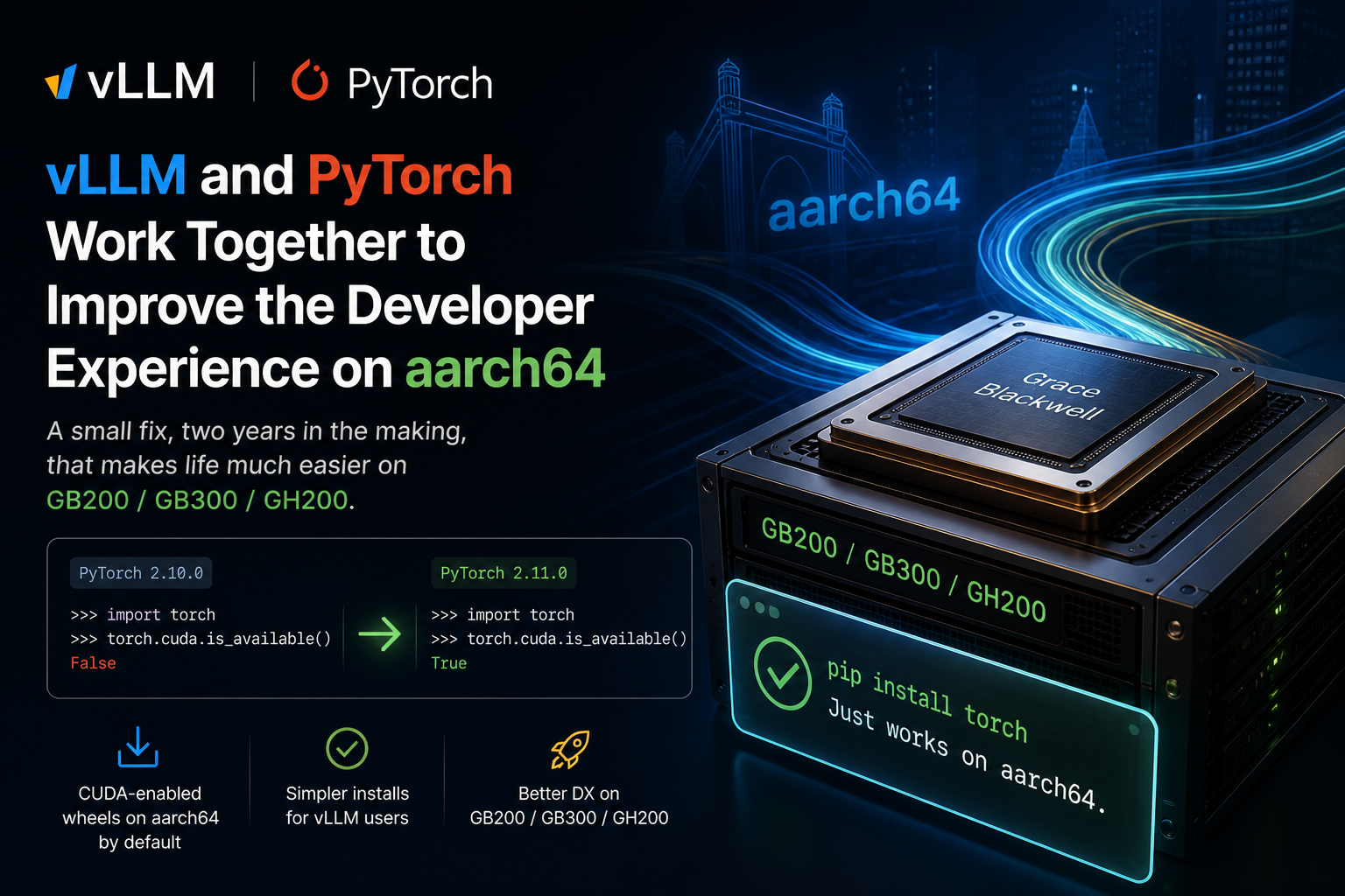
A fix, two years in the making, that makes life much easier on GB200 / GB300 / GH200.
An issue I first hit at a hackathon
This story actually starts back in October 2024.
I was at the CUDA MODE (now GPU MODE) IRL hackathon, trying to get vLLM running on a GH200 box. It should have been a five-minute job. Instead, I spent a frustrating chunk of the day staring at a pip install that, on the surface, looked perfectly fine — wheels were resolved, dependencies were satisfied, the install completed without errors — but at runtime torch.cuda.is_available() stubbornly returned False.
The reason, once I dug in, was almost comically mundane: on aarch64 Linux, pip install torch was pulling the CPU-only wheel from PyPI. There simply was no GPU wheel for aarch64 published to the default PyPI index. To get a CUDA-enabled build, you had to explicitly point pip at the PyTorch download index:
pip install torch --index-url https://download.pytorch.org/whl/cu128That, by itself, would be only mildly annoying. The real damage came from how this interacted with transitive dependencies. PyPI does not let a package specify a custom index for its dependencies. So if any package in vLLM’s dependency tree declared a requirement of torch==<some_version>, and that version doesn’t match, pip would happily go back to the default PyPI index, find the CPU wheel, silently uninstall the GPU build I had just carefully installed, and replace it with the CPU one. You’d think everything was fine until your model refused to find a GPU.
For anyone trying to bring up vLLM on GH200 — and later on GB200 / GB300 — this turned a one-line install into a maze of --index-url flags, pinned versions, and post-install sanity checks.
The workarounds vLLM carried in the meantime
While we waited for a proper fix upstream, vLLM had to ship its own workarounds so that aarch64 users were not stuck.
The first one was use_existing_torch.py, added in vllm-project/vllm#8713 back in September 2024 — explicitly framed in the PR title as “enable existing pytorch (for GH200, aarch64, nightly)”. The flow is exactly what the name suggests: you install the right torch build yourself (from the PyTorch index, or a nightly, or a custom build), then run python use_existing_torch.py, which strips every torch/torchvision/torchaudio requirement out of vLLM’s requirements/*.txt, requirements/*.in, and pyproject.toml. With those pins gone, the subsequent vLLM install can no longer trigger pip to “helpfully” reach back into the default PyPI index and silently swap your CUDA-enabled torch for the CPU wheel. It is ugly — we are literally rewriting our own dependency files at install time — but it kept GH200 users unblocked for over a year.
Later, as uv matured, we got a cleaner option. In vllm-project/vllm#24303 we added the following to pyproject.toml:
[tool.uv]
no-build-isolation-package = ["torch"]
This tells uv not to build torch in an isolated environment — which in practice means uv will reuse the torch already present in the current environment instead of trying to resolve and reinstall its own copy. Combined with installing torch first from the right index, this gave us a much more ergonomic path than the file-rewriting trick: a single config line in pyproject.toml, and uv pip install vllm (or a uv sync) would respect the pre-installed CUDA-enabled torch on aarch64.
The vLLM workaround is the community improvising around a gap in the packaging standard. Wheel Variants is NVIDIA and Astral formalizing the fix so the improvisation is no longer needed.
From a hackathon headache to a TAC agenda item
Fast forward to 2025. vLLM joined the PyTorch Foundation, and I became one of its representatives on the Technical Advisory Committee (TAC). The aarch64 wheel situation kept coming up — both in my own work and from other vLLM users on Grace Hopper and Grace Blackwell systems. In August 2025, I filed pytorch/pytorch#160162 to track the problem formally, and earlier this year, in a January 2026 TAC meeting, I raised it directly on behalf of vLLM users.
The ask was straightforward: publish aarch64 GPU wheels to the default PyPI index so that pip install torch “just works” on GB200-class machines, the same way it does on x86. Those wheels would dynamically link to libraries like NCCL and cuBLAS — the same approach already used on x86 — so they don’t balloon in size. Such large binary sizes are both hard to download for users and expensive to host by the PyPi project maintainers. Hence it is limited and heavily discouraged by the PyPi maintainer.
The Nvidia engineering team requested that the CUDA SBSA wheels be published to PyPI, and then drove the small wheel approach that links against them.
This is exactly the kind of cross-project, infrastructure-level issue that the PyTorch Foundation is well-positioned to coordinate. vLLM and PyTorch are both Foundation projects, and having a shared forum to surface ecosystem friction — rather than each project working around it independently — turned out to make a real difference.
The fix has landed
In April 2026, in another TAC meeting, I learned the issue is resolved: starting with PyTorch 2.11.0, the default pip install torch on aarch64 Linux now pulls a CUDA-enabled wheel rather than the CPU-only one. Piotr Bialecki from NVIDIA confirmed the change is live in the 2.11.0 release.
I verified it on a GB200, and the difference is exactly what you’d want — boring, in the best possible way:
$ uv run --no-project --python 3.12 --with 'torch==2.11.0' -- python -c "import torch; print(torch.cuda.is_available())"
True

$ uv run --no-project --python 3.12 --with 'torch==2.10.0' -- python -c "import torch; print(torch.cuda.is_available())"
False
One version bump, and the entire workaround stack disappears. No more custom index URLs propagating through requirements files. No more silent CPU-wheel substitutions clobbering a working install. No more “why is my GB200 not finding the GPU” debugging sessions for new users.
For vLLM specifically, this means installation on GB200 / GB300 is now genuinely smooth. New users showing up with a Grace Blackwell system can follow the standard install instructions and have things work the first time — which, when you’re trying to get inference up and running on a brand-new platform, matters a lot.
The workarounds in vLLM — both use_existing_torch.py and the [tool.uv] no-build-isolation-package = ["torch"] setting — will stay. They are still useful for advanced users who run a custom PyTorch build (a nightly, a patched fork, or a from-source build paired with a vLLM source build) and need vLLM’s install to leave that torch strictly alone. What changes is the default path: ordinary users on aarch64 no longer have to know any of this exists. They can pip install and get on with their work, and the workarounds quietly become an advanced-user tool rather than a tax on everyone.
Why this is worth writing about
It’s a small change in the grand scheme of things — a packaging tweak, not a new feature. But I think it’s worth taking a moment to appreciate, for a couple of reasons.
First, it’s a concrete example of vLLM and PyTorch collaborating productively under the PyTorch Foundation umbrella. The TAC isn’t just a governance ritual; it’s a venue where pain points from downstream projects can land in front of the people who can actually fix them, and where coordination across projects happens by default rather than by accident. This issue traveled the full path — from a developer cursing at a terminal during a hackathon, to a TAC discussion, to a tracked GitHub issue, to a release — and the Foundation is what made that path short.
Second, developer experience compounds. Every hour someone doesn’t spend wrestling with --index-url flags is an hour they spend actually building things on top of vLLM and PyTorch. aarch64 GPU systems are only going to get more common, and it’s much better to fix this now, in the boring infrastructure layer, than to leave each user to discover and work around it on their own.
The uv-side workaround (build isolation passthrough) is part of the broader WheelNext effort — a very welcome push to rethink how Python packaging handles accelerator-bound dependencies in the AI era.
A big shoutout to the people who made this happen: Alban Desmaison,Nikita Shulga, and Andrey Talman from the PyTorch core team, who picked up the original ask and helped move it through; The NVIDIA PyTorch team, who drove the aarch64 build work and confirmed the fix had landed in 2.11.0 with Piotr Bialecki supporting the effort and acting as the steady point of contact across NVIDIA and upstream on these issues; the PyTorch release engineering team for getting the wheels built and published; and the many engineers behind the scenes — across PyTorch, NVIDIA, and Arm — whose work on toolchains, CI infrastructure, and packaging made this possible. Thanks also to everyone in the TAC for keeping the door open for these kinds of conversations.
Onwards.