pytorch.org – p.41

Introducing nvFuser, a deep learning compiler for PyTorch

26 Aug 2022, 12:58 am

nvFuser is a Deep Learning Compiler for NVIDIA GPUs that automatically just-in-time compiles fast and flexible kernels to reliably accelerate users’ networks. It provides significant speedups for deep learning networks running on Volta and later CUDA accelerators by generating fast custom “fusion” kernels at runtime. nvFuser is specifically designed to meet the unique requirements of the PyTorch community, and it supports diverse network architectures and programs with dynamic inputs of varying shapes and strides. In this blog post we’ll describe nvFuser and how it’s used today, show the significant performance improvements it can obtain on models from HuggingFace and TIMM, and look ahead to nvFuser in PyTorch 1.13 and beyond. If you would like to know more about how and why fusion improves the speed of training for Deep Learning networks, please see our previous talks on nvFuser from GTC 2022 and GTC 2021. nvFuser relies on a graph representation of PyTorch operations to optimize and accelerate. Since PyTorch has an eager execution model, the PyTorch operations users are running are not directly accessible as a whole program that can be optimized by a system like nvFuser. Therefore users must utilize systems built on top of nvFuser which are capable of capturing users programs and translating them into a form that is optimizable by nvFuser. These higher level systems then pass these captured operations to nvFuser, so that nvFuser can optimize the execution of the user’s script for NVIDIA GPUs. There are three systems that capture, translate, and pass user programs to nvFuser for optimization:

• TorchScript jit.script
  • This system directly parses sections of an annotated python script to translate into its own representation what the user is doing. This system then applies its own version of auto differentiation to the graph, and passes sections of the subsequent forward and backwards graphs to nvFuser for optimization.
• FuncTorch
  • This system doesn’t directly look at the user python script, instead inserting a mechanism that captures PyTorch operations as they’re being run. We refer to this type of capture system as “trace program acquisition”, since we’re tracing what has been performed. FuncTorch doesn’t perform its own auto differentiation – it simply traces PyTorch’s autograd directly to get backward graphs.
• TorchDynamo
  • TorchDynamo is another program acquisition mechanism built on top of FuncTorch. TorchDynamo parses the Python bytecode produced from the user script in order to select portions to trace with FuncTorch. The benefit of TorchDynamo is that it’s able to apply decorators to a user’s script, effectively isolating what should be sent to FuncTorch, making it easier for FuncTorch to successfully trace complex Python scripts.

These systems are available for users to interact with directly while nvFuser automatically and seamlessly optimizes performance critical regions of the user’s code. These systems automatically send parsed user programs to nvFuser so nvFuser can:

1. Analyze the operations being run on GPUs
2. Plan parallelization and optimization strategies for those operations
3. Apply those strategies in generated GPU code
4. Runtime-compile the generated optimized GPU functions
5. Execute those CUDA kernels on subsequent iterations

It is important to note nvFuser does not yet support all PyTorch operations, and there are still some scenarios that are actively being improved in nvFuser that are discussed herein. However, nvFuser does support many DL performance critical operations today, and the number of supported operations will grow in subsequent PyTorch releases. nvFuser is capable of generating highly specialized and optimized GPU functions for the operations it does have support for. This means nvFuser is able to power new PyTorch systems like TorchDynamo and FuncTorch to combine the flexibility PyTorch is known for with unbeatable performance.

nvFuser Performance

Before getting into how to use nvFuser, in this section we’ll show the improvements in training speed nvFuser provides for a variety of models from the HuggingFace Transformers and PyTorch Image Models (TIMM) repositories and we will discuss current gaps in nvFuser performance that are under development today. All performance numbers in this section were taken using an NVIDIA A100 40GB GPU, and used either FuncTorch alone or Functorch with TorchDynamo.

HuggingFace Transformer Benchmarks

nvFuser can dramatically accelerate training of HuggingFace Transformers when combined with another important optimization (more on that in a moment). Performance improvements can be seen in Figure 1 to range between 1.12x and 1.50x across a subset of popular HuggingFace Transformer networks.

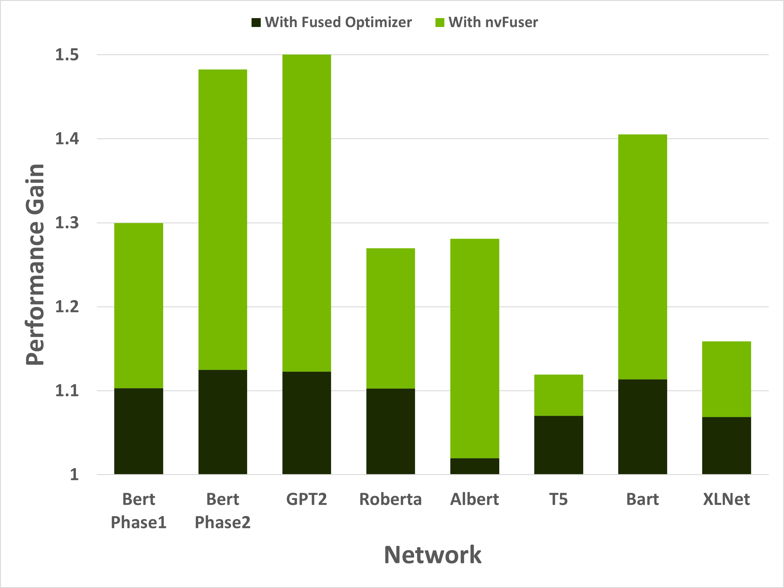
Figure 1: Performance gains of 8 training scenarios from HuggingFace’s Transformer repository. First performance boost in the dark green is due to replacing the optimizer with an NVIDIA Apex fused AdamW optimizer. The light green is due to adding nvFuser. Models were run with batch size and sequence lengths of [64, 128], [8, 512], [2, 1024], [64, 128], [8, 512], [8, src_seql=512, tgt_seql=128], [8, src_seql=1024, tgt_seql=128], and [8, 512] respectively. All networks were run with Automatic Mixed Precision (AMP) enabled with dtype=float16.

While these speedups are significant, it’s important to understand that nvFuser doesn’t (yet) automate everything about running networks quickly. For HuggingFace Transformers, for example, it was important to use the AdamW fused optimizer from NVIDIA’s Apex repository as the optimizer otherwise consumed a large portion of runtime. Using the fused AdamW optimizer to make the network faster exposes the next major performance bottleneck — memory bound operations. These operations are optimized by nvFuser, providing another large performance boost. With the fused optimizer and nvFuser enabled, the training speed of these networks improved between 1.12x to 1.5x. HuggingFace Transformer models were run with the torch.amp module. (“amp” stands for Automated Mixed Precision, see the “What Every User Should Know about Mixed Precision in PyTorch” blog post for details.) An option to use nvFuser was added to HuggingFace’sTrainer. If you have TorchDynamo installed you can activate it to enable nvFuser in HuggingFace by passing torchdynamo = ‘nvfuser’ to the Trainer class. nvFuser has great support for normalization kernels and related fusions frequently found in Natural Language Processing (NLP) models, and it is recommended users try nvFuser in their NLP workloads.

PyTorch Image Models (TIMM) Benchmarks

nvFuser, can also significantly reduce the training time of TIMM networks, up to over 1.3x vs. eager PyTorch, and up to 1.44x vs. eager PyTorch when combined with the torch.amp module. Figure 1 shows nvFuser’s speedup without torch.amp, and when torch.amp is used with the NHWC (“channels last”) and NCHW (“channels first”) formats. nvFuser is integrated in TIMM through FuncTorch tracing directly (without TorchDynamo) and can be used by adding the –aot-autograd command line argument when running the TIMM benchmark or training script.

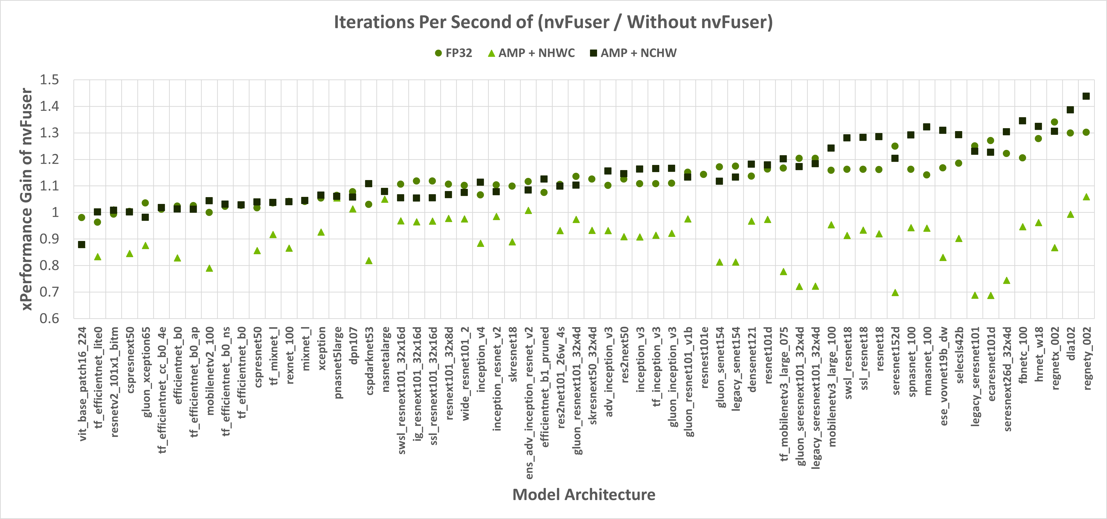
Figure 1: The Y-axis is the performance gain nvFuser provides over not using nvFuser. A value of 1.0 means no change in perf, 2.0 would mean nvFuser is twice as fast, 0.5 would mean nvFuser takes twice the time to run. Square markers are with float16 Automatic Mixed Precision (AMP) and channels first contiguous inputs, circle markers are float32 inputs, and triangles are with float16 AMP and channels last contiguous inputs. Missing data points are due to an error being encountered when tracing.

When running with float32 precision nvFuser provides a 1.12x geometric mean (“geomean”) speedup on TIMM networks, and when running with torch.amp and “channels first” it provides a 1.14x geomean speedup. However, nvFuser currently doesn’t speedup torch.amp and “channels last” training (a .9x geomean regression), so we recommend not using it in those cases. We are actively working on improving “channels last” performance now, and soon we will have two additional optimization strategies (grid persistent optimizations for channels-last normalizations and fast transposes) which we expect will provide speedups comparable to “channels first” in PyTorch version 1.13 and later. Many of nvFuser’s optimizations can also help in inference cases. However, in PyTorch when running inference on small batch sizes, the performance is typically limited by CPU overhead, which nvFuser can’t completely remove or fix. Therefore, typically the most important optimization for inference is to enable CUDA Graphs when possible. Once CUDA Graphs is enabled, then it can also be beneficial to also enable fusion through nvFuser. Performance of inference is shown in Figure 2 and Figure 3. Inference is only run with float16 AMP as it is uncommon to run inference workloads in full float32 precision.

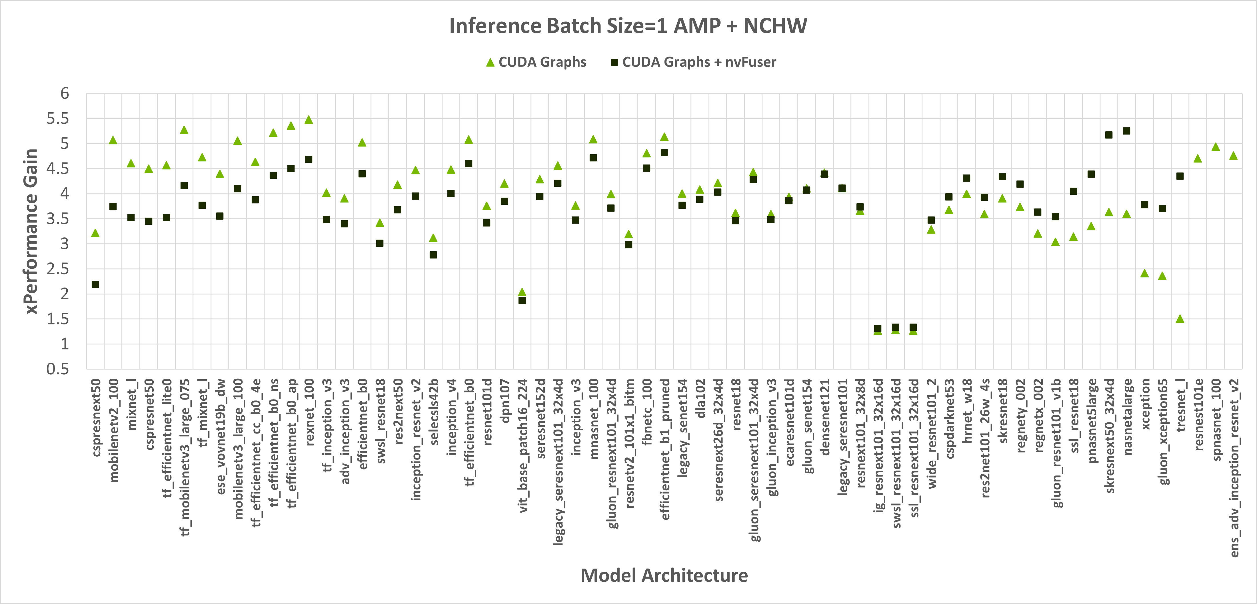
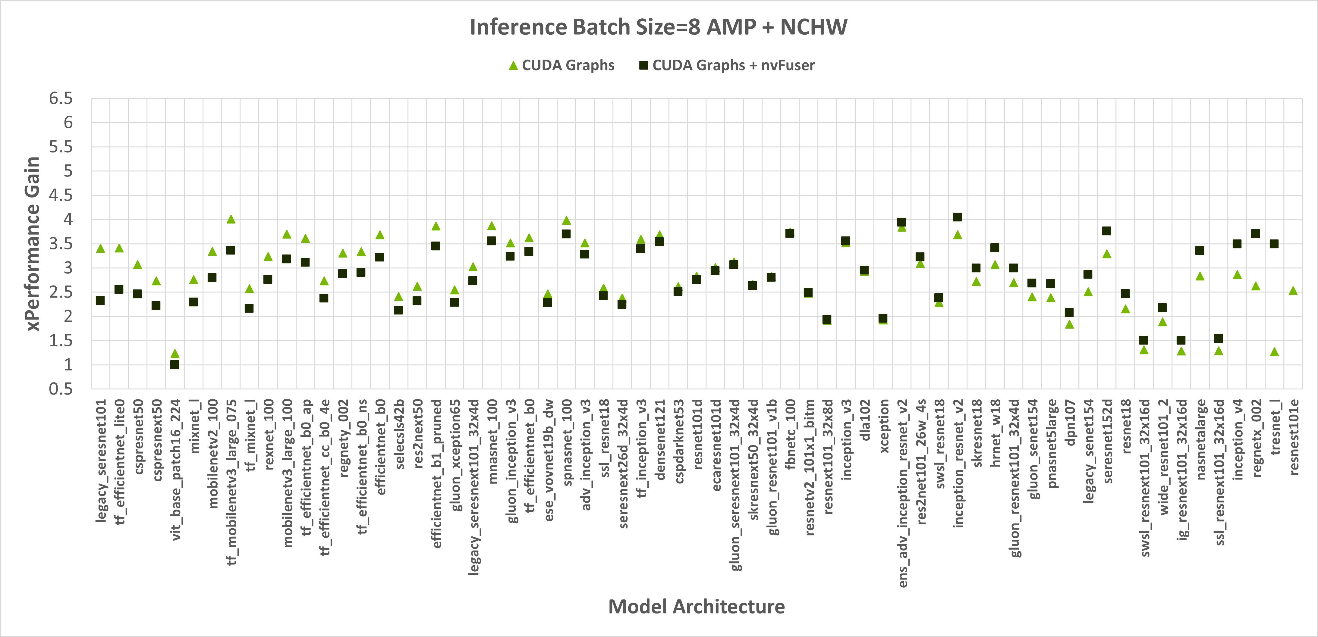
Figure 2: Performance gains of enabling CUDA Graphs, and CUDA Graphs with nvFuser compared to the performance of native PyTorch without CUDA Graphs and nvFuser across TIMM models with float16 AMP, channels first inputs, and a batch size of 1 and 8 respectively. There is a geomean speedup of 2.74x with CUDA Graphs and 2.71x with CUDA Graphs + nvFuser respectively. nvFuser provides a maximum regression of 0.68x and a maximum performance gain of 2.74x (relative to CUDA Graphs without nvFuser). Performance gain is measured relative to the average time per iteration PyTorch takes without CUDA Graphs and without nvFuser. Models are sorted by how much additional performance nvFuser is providing.

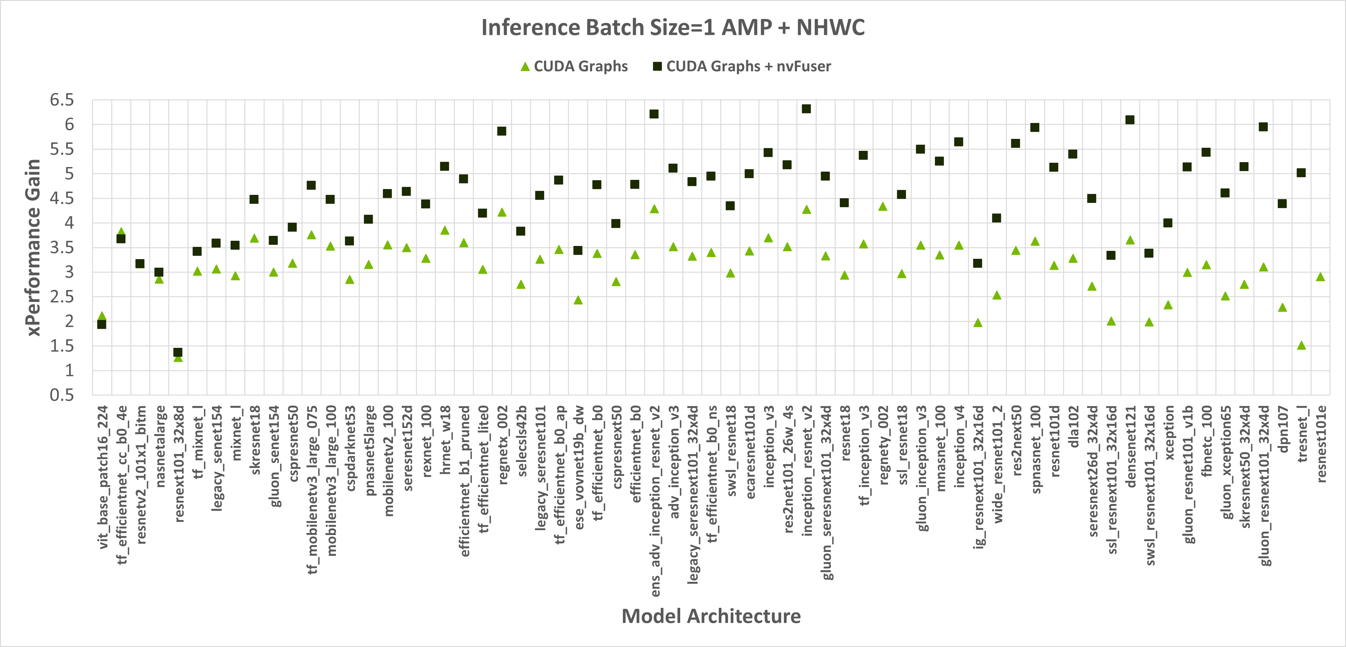
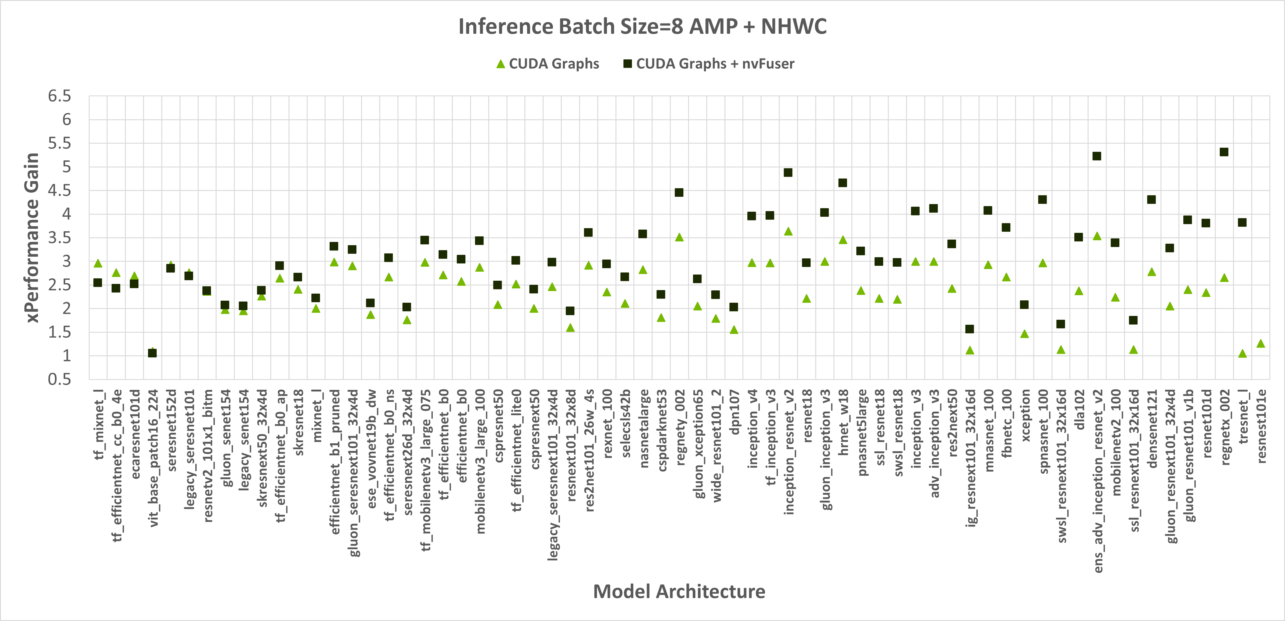
Figure 3: Performance gains of enabling CUDA Graphs, and CUDA Graphs with nvFuser compared to the performance of native PyTorch without CUDA Graphs and nvFuser across TIMM models with AMP, channels last inputs, and a batch size of 1 and 8 respectively. There is a geomean speedup of 2.29x with CUDA Graphs and 2.95x with CUDA Graphs + nvFuser respectively. nvFuser provides a maximum regression of 0.86x and a maximum performance gain of 3.82x (relative to CUDA Graphs without nvFuser). Performance gain is measured relative to the average time per iteration PyTorch takes without CUDA Graphs and without nvFuser. Models are sorted by how much additional performance nvFuser is providing.

So far nvFuser performance has not been tuned for inference workloads so its performance benefit is not consistent across all cases. However, there are still many models that benefit significantly from nvFuser during inference and we encourage users to try nvFuser in inference workloads to see if you would benefit today. Performance of nvFuser in inference workloads will improve in the future and if you’re interested in nvFuser in inference workloads please reach out to us on the PyTorch forums.

Getting Started – Accelerate Your Scripts with nvFuser

We’ve created a tutorial demonstrating how to take advantage of nvFuser to accelerate part of a standard transformer block, and how nvFuser can be used to define fast and novel operations. There are still some rough edges in nvFuser that we’re working hard on improving as we’ve outlined in this blog post. However we’ve also demonstrated some great improvements for training speed on multiple networks in HuggingFace and TIMM and we expect there are opportunities in your networks where nvFuser can help today, and many more opportunities it will help in the future. If you would like to learn more about nvFuser we recommend watching our presentations from NVIDIA’s GTC conference GTC 2022 and GTC 2021.

Accelerating PyTorch Vision Models with Channels Last on CPU

24 Aug 2022, 1:02 am

Overview

Memory formats has significant impact on performance when running vision models, generally Channels Last is a more favorable from performance perspective due to better data locality.

This blog will introduce fundamental concepts of memory formats and demonstrate performance benefits using Channels Last on popular PyTorch vision models on Intel® Xeon® Scalable processors.

Memory Formats Introduction

Memory format refers to data representation that describes how a multidimensional (nD) array is stored in linear (1D) memory address space. The concept of memory format has two aspects:

• Physical Order is the layout of data storage in physical memory. For vision models, usually we talk about NCHW, NHWC. These are the descriptions of physical memory layout, also referred as Channels First and Channels Last respectively.
• Logical Order is a convention on how to describe tensor shape and stride. In PyTorch, this convention is NCHW. No matter what the physical order is, tensor shape and stride will always be depicted in the order of NCHW.

Fig-1 is the physical memory layout of a tensor with shape of [1, 3, 4, 4] on both Channels First and Channels Last memory format (channels denoted as R, G, B respectively):

Fig-1 Physical memory layout of Channels First and Channels Last

Memory Formats Propagation

The general rule for PyTorch memory format propagation is to preserve the input tensor’s memory format. Which means a Channels First input will generate a Channels First output and a Channels Last input will generate a Channels Last output.

For Convolution layers, PyTorch uses oneDNN (oneAPI Deep Neural Network Library) by default to achieve optimal performance on Intel CPUs. Since it is physically impossible to achieve highly optimized performance directly with Channels Frist memory format, input and weight are firstly converted to blocked format and then computed. oneDNN may choose different blocked formats according to input shapes, data type and hardware architecture, for vectorization and cache reuse purposes. The blocked format is opaque to PyTorch, so the output needs to be converted back to Channels First. Though blocked format would bring about optimal computing performance, the format conversions may add overhead and therefore offset the performance gain.

On the other hand, oneDNN is optimized for Channels Last memory format to use it for optimal performance directly and PyTorch will simply pass a memory view to oneDNN. Which means the conversion of input and output tensor is saved. Fig-2 indicates memory format propagation behavior of convolution on PyTorch CPU (the solid arrow indicates a memory format conversion, and the dashed arrow indicates a memory view):

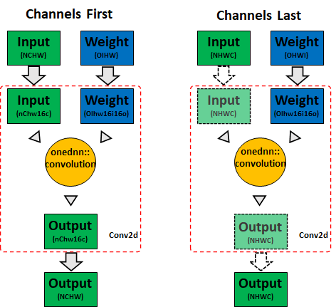
Fig-2 CPU Conv memory format propagation

On PyTorch, the default memory format is Channels First. In case a particular operator doesn’t have support on Channels Last, the NHWC input would be treated as a non-contiguous NCHW and therefore fallback to Channels First, which will consume the previous memory bandwidth on CPU and result in suboptimal performance.

Therefore, it is very important to extend the scope of Channels Last support for optimal performance. And we have implemented Channels Last kernels for the commonly use operators in CV domain, applicable for both inference and training, such as:

• Activations (e.g., ReLU, PReLU, etc.)
• Convolution (e.g., Conv2d)
• Normalization (e.g., BatchNorm2d, GroupNorm, etc.)
• Pooling (e.g., AdaptiveAvgPool2d, MaxPool2d, etc.)
• Shuffle (e.g., ChannelShuffle, PixelShuffle)

Refer to Operators-with-Channels-Last-support for details.

Native Level Optimization on Channels Last

As mentioned above, PyTorch uses oneDNN to achieve optimal performance on Intel CPUs for convolutions. The rest of memory format aware operators are optimized at PyTorch native level, which doesn’t require any third-party library support.

• Cache friendly parallelization scheme: keep the same parallelization scheme for all the memory format aware operators, this will help increase data locality when passing each layer’s output to the next.
• Vectorization on multiple archs: generally, we can vectorize on the most inner dimension on Channels Last memory format. And each of the vectorized CPU kernels will be generated for both AVX2 and AVX512.

While contributing to Channels Last kernels, we tried our best to optimize Channels First counterparts as well. The fact is some operators are physically impossible to achieve optimal performance on Channels First, such as Convolution, Pooling, etc.

Run Vision Models on Channels Last

The Channels Last related APIs are documented at PyTorch memory format tutorial. Typically, we can convert a 4D tensor from Channels First to Channels Last by:

# convert x to channels last
# suppose x’s shape is (N, C, H, W)
# then x’s stride will be (HWC, 1, WC, C)
x = x.to(memory_format=torch.channels_last)

To run models on Channels Last memory format, simply need to convert input and model to Channels Last and then you are ready to go. The following is a minimal example showing how to run ResNet50 with TorchVision on Channels Last memory format:

import torch
from torchvision.models import resnet50

N, C, H, W = 1, 3, 224, 224
x = torch.rand(N, C, H, W)
model = resnet50()
model.eval()

# convert input and model to channels last
x = x.to(memory_format=torch.channels_last)
model = model.to(memory_format=torch.channels_last)
model(x)

The Channels Last optimization is implemented at native kernel level, which means you may apply other functionalities such as torch.fx and torch script together with Channels Last as well.

Performance Gains

We benchmarked inference performance of TorchVision models on Intel® Xeon® Platinum 8380 CPU @ 2.3 GHz, single instance per socket (batch size = 2 x number of physical cores). Results show that Channels Last has 1.3x to 1.8x performance gain over Channels First.

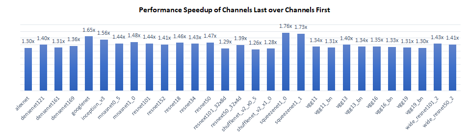
The performance gain primarily comes from two aspects:

• For Convolution layers, Channels Last saved the memory format conversion to blocked format for activations, which improves the overall computation efficiency.
• For Pooling and Upsampling layers, Channels Last can use vectorized logic along the most inner dimension, e.g., “C”, while Channels First can’t.

For memory format non aware layers, Channels Last and Channels First has the same performance.

Conclusion & Future Work

In this blog we introduced fundamental concepts of Channels Last and demonstrated the performance benefits of CPU using Channels Last on vision models. The current work is limited to 2D models at the current stage, and we will extend the optimization effort to 3D models in near future!

Acknowledgement

The results presented in this blog is a joint effort of Meta and Intel PyTorch team. Special thanks to Vitaly Fedyunin and Wei Wei from Meta who spent precious time and gave substantial assistance! Together we made one more step on the path of improving the PyTorch CPU eco system.

References

• PyTorch memory format tutorial
• oneDNN guide on memory formats
• PyTorch operators with Channels Last support

Easily list and initialize models with new APIs in TorchVision

18 Aug 2022, 1:06 am

TorchVision now supports listing and initializing all available built-in models and weights by name. This new API builds upon the recently introduced Multi-weight support API, is currently in Beta, and it addresses a long-standing request from the community.

You can try out the new API in the latest nightly release of TorchVision. We’re looking to collect feedback ahead of finalizing the feature in TorchVision v0.14. We have created a dedicated Github Issue where you can post your comments, questions and suggestions!

Querying and initializing available models

Before the new model registration API, developers had to query the __dict__ attribute of the modules in order to list all available models or to fetch a specific model builder method by its name:

# Initialize a model by its name:
model = torchvision.models.__dict__[model_name]()

# List available models:
available_models = [
    k for k, v in torchvision.models.__dict__.items()
    if callable(v) and k[0].islower() and k[0] != "_"
]

The above approach does not always produce the expected results and is hard to discover. For example, since the get_weight() method is exposed publicly under the same module, it will be included in the list despite not being a model. In general, reducing the verbosity (less imports, shorter names etc) and being able to initialize models and weights directly from their names (better support of configs, TorchHub etc) was feedback provided previously by the community. To solve this problem, we have developed a model registration API.

A new approach

We’ve added 4 new methods under the torchvision.models module:

from torchvision.models import get_model, get_model_weights, get_weight, list_models

The styles and naming conventions align closely with a prototype mechanism proposed by Philip Meier for the Datasets V2 API, aiming to offer a similar user experience. The model registration methods are kept private on purpose as we currently focus only on supporting the built-in models of TorchVision.

List models

Listing all available models in TorchVision can be done with a single function call:

>>> list_models()
['alexnet', 'mobilenet_v3_large', 'mobilenet_v3_small', 'quantized_mobilenet_v3_large', ...]

To list the available models of specific submodules:

>>> list_models(module=torchvision.models)
['alexnet', 'mobilenet_v3_large', 'mobilenet_v3_small', ...]
>>> list_models(module=torchvision.models.quantization)
['quantized_mobilenet_v3_large', ...]

Initialize models

Now that you know which models are available, you can easily initialize a model with pre-trained weights:

>>> get_model("quantized_mobilenet_v3_large", weights="DEFAULT")
QuantizableMobileNetV3(
  (features): Sequential(
   ....
   )
)

Get weights

Sometimes, while working with config files or using TorchHub, you might have the name of a specific weight entry and wish to get its instance. This can be easily done with the following method:

>>> get_weight("ResNet50_Weights.IMAGENET1K_V2")
ResNet50_Weights.IMAGENET1K_V2

To get the enum class with all available weights of a specific model you can use either its name:

>>> get_model_weights("quantized_mobilenet_v3_large")
<enum 'MobileNet_V3_Large_QuantizedWeights'>

Or its model builder method:

>>> get_model_weights(torchvision.models.quantization.mobilenet_v3_large)
<enum 'MobileNet_V3_Large_QuantizedWeights'>

TorchHub support

The new methods are also available via TorchHub:

import torch

# Fetching a specific weight entry by its name:
weights = torch.hub.load("pytorch/vision", "get_weight", weights="ResNet50_Weights.IMAGENET1K_V2")

# Fetching the weights enum class to list all available entries:
weight_enum = torch.hub.load("pytorch/vision", "get_model_weights", name="resnet50")
print([weight for weight in weight_enum])

Putting it all together

For example, if you wanted to retrieve all the small-sized models with pre-trained weights and initialize one of them, it’s a matter of using the above APIs:

import torchvision
from torchvision.models import get_model, get_model_weights, list_models


max_params = 5000000

tiny_models = []
for model_name in list_models(module=torchvision.models):
    weights_enum = get_model_weights(model_name)
    if len([w for w in weights_enum if w.meta["num_params"] <= max_params]) > 0:
        tiny_models.append(model_name)

print(tiny_models)
# ['mnasnet0_5', 'mnasnet0_75', 'mnasnet1_0', 'mobilenet_v2', ...]

model = get_model(tiny_models[0], weights="DEFAULT")
print(sum(x.numel() for x in model.state_dict().values()))
# 2239188

For more technical details please see the original RFC. Please spare a few minutes to provide your feedback on the new API, as this is crucial for graduating it from beta and including it in the next release. You can do this on the dedicated Github Issue. We are looking forward to reading your comments!

Empowering PyTorch on Intel® Xeon® Scalable processors with Bfloat16

16 Aug 2022, 1:08 am

Overview

Recent years, the growing complexity of AI models have been posing requirements on hardware for more and more compute capability. Reduced precision numeric format has been proposed to address this problem. Bfloat16 is a custom 16-bit floating point format for AI which consists of one sign bit, eight exponent bits, and seven mantissa bits. With the same dynamic range as float32, bfloat16 doesn’t require a special handling such as loss scaling. Therefore, bfloat16 is a drop-in replacement for float32 when running deep neural networks for both inference and training.

The 3rd Gen Intel^® Xeon^® Scalable processor (codenamed Cooper Lake), is the first general purpose x86 CPU with native bfloat16 support. Three new bfloat16 instructions were introduced in Intel^® Advanced Vector Extensions-512 (Intel^® AVX-512): VCVTNE2PS2BF16, VCVTNEPS2BF16, and VDPBF16PS. The first two instructions perform conversion from float32 to bfloat16, and the last one performs a dot product of bfloat16 pairs. Bfloat16 theoretical compute throughput is doubled over float32 on Cooper Lake. On the next generation of Intel^® Xeon^® Scalable Processors, bfloat16 compute throughput will be further enhanced through Advanced Matrix Extensions (Intel^® AMX) instruction set extension.

Intel and Meta previously collaborated to enable bfloat16 on PyTorch, and the related work was published in an earlier blog during launch of Cooper Lake. In that blog, we introduced the hardware advancement for native bfloat16 support and showcased a performance boost of 1.4x to 1.6x of bfloat16 over float32 from DLRM, ResNet-50 and ResNext-101-32x4d.

In this blog, we will introduce the latest software enhancement on bfloat16 in PyTorch 1.12, which would apply to much broader scope of user scenarios and showcase even higher performance boost.

Native Level Optimization on Bfloat16

On PyTorch CPU bfloat16 path, the compute intensive operators, e.g., convolution, linear and bmm, use oneDNN (oneAPI Deep Neural Network Library) to achieve optimal performance on Intel CPUs with AVX512_BF16 or AMX support. The other operators, such as tensor operators and neural network operators, are optimized at PyTorch native level. We have enlarged bfloat16 kernel level optimizations to majority of operators on dense tensors, both inference and training applicable (sparse tensor bfloat16 support will be covered in future work), specifically:

• Bfloat16 vectorization: Bfloat16 is stored as unsigned 16-bit integer, which requires it to be casted to float32 for arithmetic operations such as add, mul, etc. Specifically, each bfloat16 vector will be converted to two float32 vectors, processed accordingly and then converted back. While for non-arithmetic operations such as cat, copy, etc., it is a straight memory copy and no data type conversion will be involved.
• Bfloat16 reduction: Reduction on bfloat16 data uses float32 as accumulation type to guarantee numerical stability, e.g., sum, BatchNorm2d, MaxPool2d, etc.
• Channels Last optimization: For vision models, Channels Last is the preferable memory format over Channels First from performance perspective. We have implemented fully optimized CPU kernels for all the commonly used CV modules on channels last memory format, taking care of both float32 and bfloat16.

Run Bfloat16 with Auto Mixed Precision

To run model on bfloat16, typically user can either explicitly convert the data and model to bfloat16, for example:

# with explicit conversion
input = input.to(dtype=torch.bfloat16)
model = model.to(dtype=torch.bfloat16)

or utilize torch.amp (Automatic Mixed Precision) package. The autocast instance serves as context managers or decorators that allow regions of your script to run in mixed precision, for example:

# with AMP
with torch.autocast(device_type="cpu", dtype=torch.bfloat16):
    output = model(input)

Generally, the explicit conversion approach and AMP approach have similar performance. Even though, we recommend run bfloat16 models with AMP, because:

• Better user experience with automatic fallback: If your script includes operators that don’t have bfloat16 support, autocast will implicitly convert them back to float32 while the explicit converted model will give a runtime error.
• Mixed data type for activation and parameters: Unlike the explicit conversion which converts all the model parameters to bfloat16, AMP mode will run in mixed data type. To be specific, input/output will be kept in bfloat16 while parameters, e.g., weight/bias, will be kept in float32. The mixed data type of activation and parameters will help improve performance while maintaining the accuracy.

Performance Gains

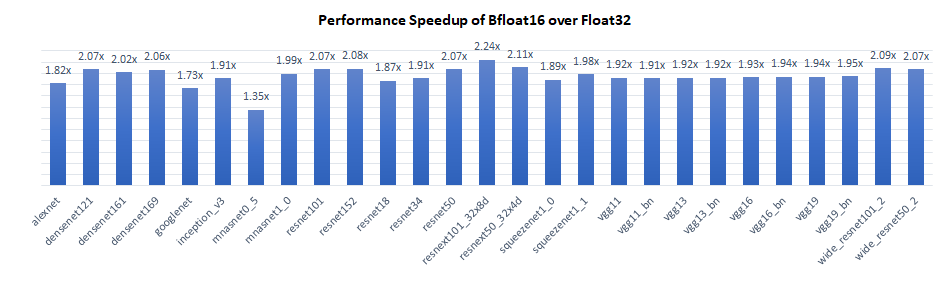
We benchmarked inference performance of TorchVision models on Intel® Xeon® Platinum 8380H CPU @ 2.90GHz (codenamed Cooper Lake), single instance per socket (batch size = 2 x number of physical cores). Results show that bfloat16 has 1.4x to 2.2x performance gain over float32.

The performance boost of bfloat16 over float32 primarily comes from 3 aspects:

• The compute intensive operators take advantage of the new bfloat16 native instruction VDPBF16PS which doubles the hardware compute throughput.
• Bfloat16 have only half the memory footprint of float32, so theoretically the memory bandwidth intensive operators will be twice faster.
• On Channels Last, we intentionally keep the same parallelization scheme for all the memory format aware operators (can’t do this on Channels First though), which increases the data locality when passing each layer’s output to the next. Basically, it keeps the data closer to CPU cores while data would reside in cache anyway. And bfloat16 will have a higher cache hit rate compared with float32 in such scenarios due to smaller memory footprint.

Conclusion & Future Work

In this blog, we introduced recent software optimizations on bfloat16 introduced in PyTorch 1.12. Results on the 3rd Gen Intel^® Xeon^® Scalable processor show that bfloat16 has 1.4x to 2.2x performance gain over float32 on the TorchVision models. Further improvement is expected on the next generation of Intel^® Xeon^® Scalable Processors with AMX instruction support. Though the performance number for this blog is collected with TorchVision models, the benefit is broad across all topologies. And we will continue to extend the bfloat16 optimization effort to a broader scope in the future!

Acknowledgement

The results presented in this blog is a joint effort of Meta and Intel PyTorch team. Special thanks to Vitaly Fedyunin and Wei Wei from Meta who spent precious time and gave substantial assistance! Together we made one more step on the path of improving the PyTorch CPU eco system.

Reference

• The bfloat16 numerical format
• https://pytorch.org/docs/master/amp.html#torch.autocast
• Intel and Facebook Accelerate PyTorch Performance with 3rd Gen Intel® Xeon® Processors and Intel® Deep Learning Boost’s new BFloat16 capability

Introducing the PlayTorch app: Rapidly Create Mobile AI Experiences

22 Jul 2022, 1:09 am

In December, we announced PyTorch Live, a toolkit for building AI-powered mobile prototypes in minutes. The initial release included a command-line interface to set up a development environment and an SDK for building AI-powered experiences in React Native. Today, we’re excited to share that PyTorch Live will now be known as PlayTorch. This new release provides an improved and simplified developer experience. PlayTorch development is independent from the PyTorch project and the PlayTorch code repository is moving into the Meta Research GitHub organization.

A New Workflow: The PlayTorch App

The PlayTorch team is excited to announce that we have partnered with Expo to change the way AI powered mobile experiences are built. Our new release simplifies the process of building mobile AI experiences by eliminating the need for a complicated development environment. You will now be able to build cross platform AI powered prototypes from the very browser you are using to read this blog.

In order to make this happen, we are releasing the PlayTorch app which is able to run AI-powered experiences built in the Expo Snack web based code editor.

The PlayTorch app can be downloaded from the Apple App Store and Google Play Store. With the app installed, you can head over to playtorch.dev/snack and write the code for your AI-powered PlayTorch Snack. When you want to try what you’ve built, you can use the PlayTorch app’s QR code scanner to scan the QR code on the Snack page and load the code to your device.

NOTE: PlayTorch Snacks will not work in the Expo Go app.

More to Explore in the PlayTorch App

AI Demos

The PlayTorch app comes with several examples of how you can build AI powered experiences with a variety of different machine learning models from object detection to natural language processing. See what can be built with the PlayTorch SDK and be inspired to make something of your own as you play with the examples.

Sharing Your Creations

Any PlayTorch Snack that you run in the PlayTorch app can be shared with others in an instant. When they open the link on their device, the PlayTorch app will instantly load what you’ve built from the cloud so they can experience it first hand.

When you have something you want to share, let us know on Discord or Twitter or embed the PlayTorch Snack on your own webpage.

SDK Overhaul

We learned a lot from the community after our initial launch in December and have been hard at work over the past several months to make the PlayTorch SDK (formerly known as PyTorch Live) simple, performant, and robust. In our initial version, the SDK relied on config files to define how a model ingested and output data.

Today, we are happy to announce the next version of our SDK can handle data processing in JavaScript for your prototypes with the new PlayTorch API that leverages the JavaScript Interface (JSI) to directly call C++ code. Not only have we completely redone the way you can interact with models, but we have also greatly expanded the variety of supported model architectures.

A New Data Processing API for Prototyping

With this JSI API, we now allow users direct access to tensors (data format for machine learning). Instead of only having access to predefined transformations, you can now manipulate tensors however you would like for your prototypes.

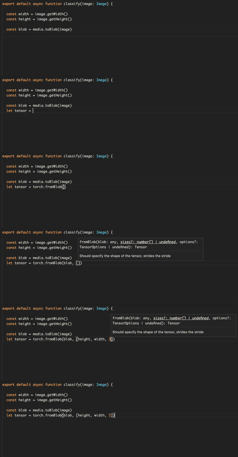
No more switching back and forth between code and config. You will now be able to write everything in JavaScript and have access to all of the type annotations and autocomplete features available to you in those languages.

Check out our tutorials to see the new Data Processing API in action, take a deeper dive in the API docs, or inspect the code yourself on GitHub.

Expanded Use Cases

With the new version of the SDK, we have added support for several cutting edge models.

Image-to-image transformations are now supported thanks to our robust JSI API, so you can see what your world would look like if it were an anime.

Translate French to English with an AI powered translator using the Seq2Seq model.

Use DeepLab V3 to segment images!

Start Playing

If you want to start creating AI experiences yourself, head over to playtorch.dev and try out our tutorials. Each tutorial will guide you through building a simple AI powered experience that you can instantly run on your phone and share with others.

How to Get Support

Join us on Discord, collaborate with us on GitHub, or follow us on Twitter. Got questions or feedback? We’d love to hear from you!

What Every User Should Know About Mixed Precision Training in PyTorch

19 Jul 2022, 1:14 am

Efficient training of modern neural networks often relies on using lower precision data types. Peak float16 matrix multiplication and convolution performance is 16x faster than peak float32 performance on A100 GPUs. And since the float16 and bfloat16 data types are only half the size of float32 they can double the performance of bandwidth-bound kernels and reduce the memory required to train a network, allowing for larger models, larger batches, or larger inputs. Using a module like torch.amp (short for “Automated Mixed Precision”) makes it easy to get the speed and memory usage benefits of lower precision data types while preserving convergence behavior.

Going faster and using less memory is always advantageous – deep learning practitioners can test more model architectures and hyperparameters, and larger, more powerful models can be trained. Training very large models like those described in Narayanan et al. and Brown et al. (which take thousands of GPUs months to train even with expert handwritten optimizations) is infeasible without using mixed precision.

We’ve talked about mixed precision techniques before (here, here, and here), and this blog post is a summary of those techniques and an introduction if you’re new to mixed precision.

Mixed Precision Training in Practice

Mixed precision training techniques – the use of the lower precision float16 or bfloat16 data types alongside the float32 data type – are broadly applicable and effective. See Figure 1 for a sampling of models successfully trained with mixed precision, and Figures 2 and 3 for example speedups using torch.amp.

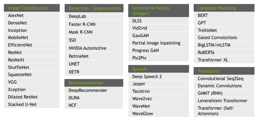
Figure 1: Sampling of DL Workloads Successfully Trained with float16 (Source).

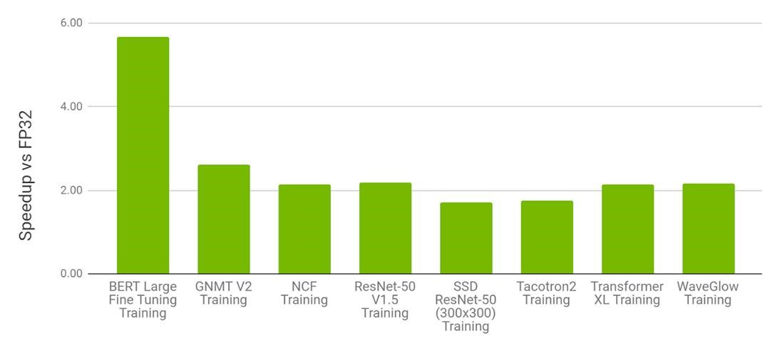
Figure 2: Performance of mixed precision training using torch.amp on NVIDIA 8xV100 vs. float32 training on 8xV100 GPU. Bars represent the speedup factor of torch.amp over float32. (Higher is better.) (Source).

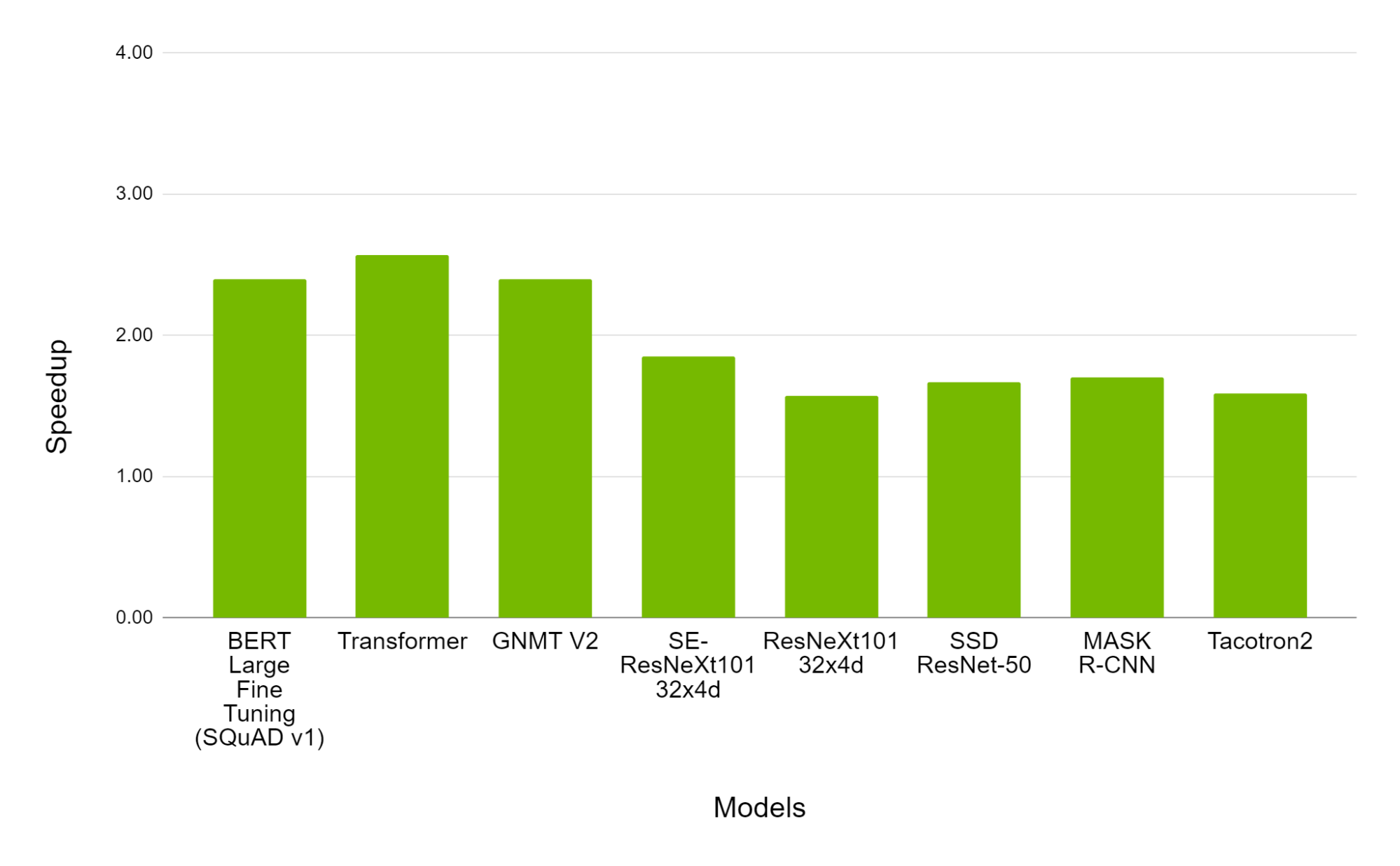
Figure 3. Performance of mixed precision training using torch.amp on NVIDIA 8xA100 vs. 8xV100 GPU. Bars represent the speedup factor of A100 over V100. (Higher is Better.) (Source).

See the NVIDIA Deep Learning Examples repository for more sample mixed precision workloads.

Similar performance charts can be seen in 3D medical image analysis, gaze estimation, video synthesis, conditional GANs, and convolutional LSTMs. Huang et al. showed that mixed precision training is 1.5x to 5.5x faster over float32 on V100 GPUs, and an additional 1.3x to 2.5x faster on A100 GPUs on a variety of networks. On very large networks the need for mixed precision is even more evident. Narayanan et al. reports that it would take 34 days to train GPT-3 175B on 1024 A100 GPUs (with a batch size of 1536), but it’s estimated it would take over a year using float32!

Getting Started With Mixed Precision Using torch.amp

torch.amp, introduced in PyTorch 1.6, makes it easy to leverage mixed precision training using the float16 or bfloat16 dtypes. See this blog post, tutorial, and documentation for more details. Figure 4 shows an example of applying AMP with grad scaling to a network.

import torch
# Creates once at the beginning of training
scaler = torch.cuda.amp.GradScaler()

for data, label in data_iter:
   optimizer.zero_grad()
   # Casts operations to mixed precision
   with torch.amp.autocast(device_type=“cuda”, dtype=torch.float16):
      loss = model(data)

   # Scales the loss, and calls backward()
   # to create scaled gradients
   scaler.scale(loss).backward()

   # Unscales gradients and calls
   # or skips optimizer.step()
   scaler.step(optimizer)

   # Updates the scale for next iteration
   scaler.update()

Figure 4: AMP recipe

Picking The Right Approach

Out-of-the-box mixed precision training with either float16 or bfloat16 is effective at speeding up the convergence of many deep learning models, but some models may require more careful numerical accuracy management. Here are some options:

• Full float32 precision. Floating point tensors and modules are created in float32 precision by default in PyTorch, but this is a historic artifact not representative of training most modern deep learning networks. It’s rare that networks need this much numerical accuracy.
• Enabling TensorFloat32 (TF32) mode. On Ampere and later CUDA devices matrix multiplications and convolutions can use the TensorFloat32 (TF32) mode for faster but slightly less accurate computations. See the Accelerating AI Training with NVIDIA TF32 Tensor Cores blog post for more details. By default PyTorch enables TF32 mode for convolutions but not matrix multiplications, and unless a network requires full float32 precision we recommend enabling this setting for matrix multiplications, too (see the documentation here for how to do so). It can significantly speed up computations with typically negligible loss of numerical accuracy.
• Using torch.amp with bfloat16 or float16. Both these low precision floating point data types are usually comparably fast, but some networks may only converge with one vs the other. If a network requires more precision it may need to use float16, and if a network requires more dynamic range it may need to use bfloat16, whose dynamic range is equal to that of float32. If overflows are observed, for example, then we suggest trying bfloat16.

There are even more advanced options than those presented here, like using torch.amp’s autocasting for only parts of a model, or managing mixed precision directly. These topics are largely beyond the scope of this blog post, but see the “Best Practices” section below.

Best Practices

We strongly recommend using mixed precision with torch.amp or the TF32 mode (on Ampere and later CUDA devices) whenever possible when training a network. If one of those approaches doesn’t work, however, we recommend the following:

• High Performance Computing (HPC) applications, regression tasks, and generative networks may simply require full float32 IEEE precision to converge as expected.
• Try selectively applying torch.amp. In particular we recommend first disabling it on regions performing operations from the torch.linalg module or when doing pre- or post-processing. These operations are often especially sensitive. Note that TF32 mode is a global switch and can’t be used selectively on regions of a network. Enable TF32 first to check if a network’s operators are sensitive to the mode, otherwise disable it.
• If you encounter type mismatches while using torch.amp we don’t suggest inserting manual casts to start. This error is indicative of something being off with the network, and it’s usually worth investigating first.
• Figure out by experimentation if your network is sensitive to range and/or precision of a format. For example fine-tuning bfloat16-pretrained models in float16 can easily run into range issues in float16 because of the potentially large range from training in bfloat16, so users should stick with bfloat16 fine-tuning if the model was trained in bfloat16.
• The performance gain of mixed precision training can depend on multiple factors (e.g. compute-bound vs memory-bound problems) and users should use the tuning guide to remove other bottlenecks in their training scripts. Although having similar theoretical performance benefits, BF16 and FP16 can have different speeds in practice. It’s recommended to try the mentioned formats and use the one with best speed while maintaining the desired numeric behavior.

For more details, refer to the AMP Tutorial, Training Neural Networks with Tensor Cores, and see the post “More In-Depth Details of Floating Point Precision” on PyTorch Dev Discussion.

Conclusion

Mixed precision training is an essential tool for training deep learning models on modern hardware, and it will become even more important in the future as the performance gap between lower precision operations and float32 continues to grow on newer hardware, as reflected in Figure 5.

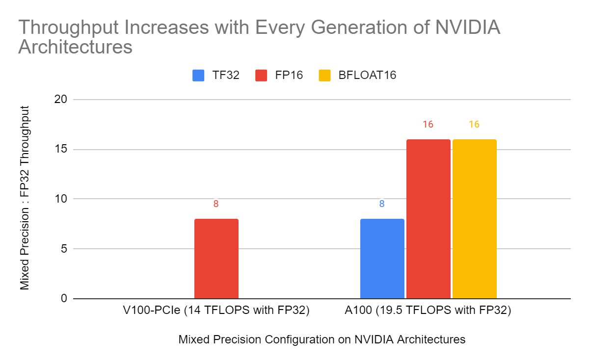
Figure 5: Relative peak throughput of float16 (FP16) vs float32 matrix multiplications on Volta and Ampere GPUs. On Ampere relative peak throughput for the TensorFloat32 (TF32) mode and bfloat16 matrix multiplications are shown, too. The relative peak throughput of low precision data types like float16 and bfloat16 vs. float32 matrix multiplications is expected to grow as new hardware is released.

PyTorch’s torch.amp module makes it easy to get started with mixed precision, and we highly recommend using it to train faster and reduce memory usage. torch.amp supports both float16 and bfloat16 mixed precision.

There are still some networks that are tricky to train with mixed precision, and for these networks we recommend trying TF32 accelerated matrix multiplications on Ampere and later CUDA hardware. Networks are rarely so precision sensitive that they require full float32 precision for every operation.

If you have questions or suggestions for torch.amp or mixed precision support in PyTorch then let us know by posting to the mixed precision category on the PyTorch Forums or filing an issue on the PyTorch GitHub page.

Case Study: PathAI Uses PyTorch to Improve Patient Outcomes with AI-powered Pathology

15 Jul 2022, 1:17 am

​​PathAI is the leading provider of AI-powered technology tools and services for pathology (the study of disease). Our platform was built to enable substantial improvements to the accuracy of diagnosis and the measurement of therapeutic efficacy for complex diseases, leveraging modern approaches in machine learning like image segmentation, graph neural networks, and multiple instance learning.

Traditional manual pathology is prone to subjectivity and observer variability that can negatively affect diagnoses and drug development trials. Before we dive into how we use PyTorch to improve our diagnosis workflow, let us first lay out the traditional analog Pathology workflow without machine learning.

How Traditional Biopharma Works

There are many avenues that biopharma companies take to discover novel therapeutics or diagnostics. One of those avenues relies heavily on the analysis of pathology slides to answer a variety of questions: how does a particular cellular communication pathway work? Can a specific disease state be linked to the presence or lack of a particular protein? Why did a particular drug in a clinical trial work for some patients but not others? Might there be an association between patient outcomes and a novel biomarker?

To help answer these questions, biopharma companies rely on expert pathologists to analyze slides and help evaluate the questions they might have. 

As you might imagine, it takes an expert board certified pathologist to make accurate interpretations and diagnosis. In one study, a single biopsy result was given to 36 different pathologists and the outcome was 18 different diagnoses varying in severity from no treatment to aggressive treatment necessary. Pathologists also often solicit feedback from colleagues in difficult edge cases. Given the complexity of the problem, even with expert training and collaboration, pathologists can still have a hard time making a correct diagnosis. This potential variance can be the difference between a drug being approved and it failing the clinical trial.

How PathAI utilizes machine learning to power drug development

PathAI develops machine learning models which provide insights for drug development R&D, for powering clinical trials, and for making diagnoses. To this end, PathAI leverages PyTorch for slide level inference using a variety of methods including graph neural networks (GNN) as well as multiple instance learning. In this context, “slides” refers to full size scanned images of glass slides, which are pieces of glass with a thin slice of tissue between them, stained to show various cell formations. PyTorch enables our teams using these different methodologies to share a common framework which is robust enough to work in all the conditions we need. PyTorch’s high level, imperative, and pythonic syntax allows us to prototype models quickly and then take those models to scale once we have the results we want. 

Multi-instance learning on gigabyte images

One of the uniquely challenging aspects of applying ML to pathology is the immense size of the images. These digital slides can often be 100,000 x 100,000 pixels or more in resolution and gigabytes in size. Loading the full image in GPU memory and applying traditional computer vision algorithms on them is an almost impossible task. It also takes both a considerable amount of time and resources to have a full slide image (100k x 100k) annotated, especially when annotators need to be domain experts (board-certified pathologists). We often build models to predict image-level labels, like the presence of cancer, on a patient slide which covers a few thousand pixels in the whole image. The cancerous area is sometimes a tiny fraction of the entire slide, which makes the ML problem similar to finding a needle in a haystack. On the other hand, some problems like the prediction of certain histological biomarkers require an aggregation of information from the whole slide which is again hard due to the size of the images. All these factors add significant algorithmic, computational, and logistical complexity when applying ML techniques to pathology problems.

Breaking down the image into smaller patches, learning patch representations, and then pooling those representations to predict an image-level label is one way to solve this problem as is depicted in the image below. One popular method for doing this is called Multiple Instance Learning (MIL). Each patch is considered an ‘instance’ and a set of patches forms a ‘bag’. The individual patch representations are pooled together to predict a final bag-level label. Algorithmically, the individual patch instances in the bag do not require labels and hence allow us to learn bag-level labels in a weakly-supervised way. They also use permutation invariant pooling functions which make the prediction independent of the order of patches and allows for an efficient aggregation of information. Typically, attention based pooling functions are used which not only allow for efficient aggregation but also provide attention values for each patch in the bag. These values indicate the importance of the corresponding patch in the prediction and can be visualized to better understand the model predictions. This element of interpretability can be very important to drive adoption of these models in the real world and we use variations like Additive MIL models to enable such spatial explainability. Computationally, MIL models circumvent the problem of applying neural networks to large image sizes since patch representations are obtained independently of the size of the image.

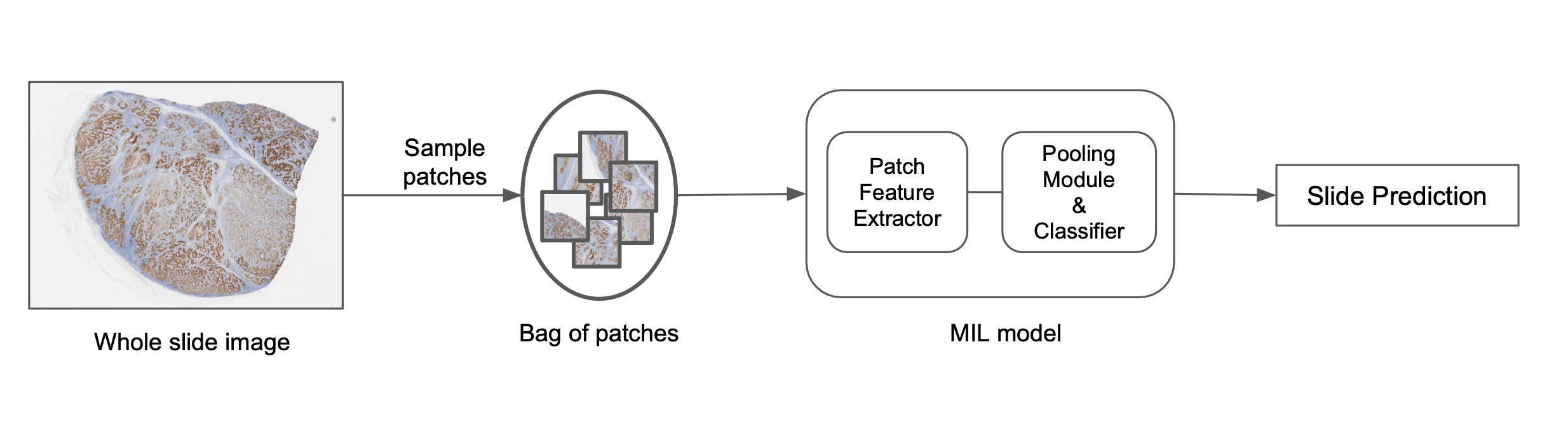
At PathAI, we use custom MIL models based on deep nets to predict image-level labels. The overview of this process is as follows:

1. Select patches from a slide using different sampling approaches.
2. Construct a bag of patches based on random sampling or heuristic rules.
3. Generate patch representations for each instance based on pre-trained models or large-scale representation learning models.
4. Apply permutation invariant pooling functions to get the final slide-level score.

Now that we have walked through some of the high-level details around MIL in PyTorch, let’s look at some code to see how simple it is to go from ideation to code in production with PyTorch. We begin by defining a sampler, transformations, and our MIL dataset:

# Create a bag sampler which randomly samples patches from a slide
bag_sampler = RandomBagSampler(bag_size=12)

# Setup the transformations
crop_transform = FlipRotateCenterCrop(use_flips=True)

# Create the dataset which loads patches for each bag
train_dataset = MILDataset(
  bag_sampler=bag_sampler,
  samples_loader=sample_loader,
  transform=crop_transform,
)

After we have defined our sampler and dataset, we need to define the model we will actually train with said dataset. PyTorch’s familiar model definition syntax makes this easy to do while also allowing us to create bespoke models at the same time.

classifier = DefaultPooledClassifier(hidden_dims=[256, 256], input_dims=1024, output_dims=1)

pooling = DefaultAttentionModule(
  input_dims=1024,
  hidden_dims=[256, 256],
  output_activation=StableSoftmax()
)

# Define the model which is a composition of the featurizer, pooling module and a classifier
model = DefaultMILGraph(featurizer=ShuffleNetV2(), classifier=classifier, pooling = pooling)

Since these models are trained end-to-end, they offer a powerful way to go directly from a gigapixel whole slide image to a single label. Due to their wide applicability to different biological problems, two aspects of their implementation and deployment are important:

1. Configurable control over each part of the pipeline including the data loaders, the modular parts of the model, and their interaction with each other.
2. Ability to rapidly iterate through the ideate-implement-experiment-productionize loop.

PyTorch has various advantages when it comes to MIL modeling. It offers an intuitive way to create dynamic computational graphs with flexible control flow which is great for rapid research experimentation. The map-style datasets, configurable sampler and batch-samplers allow us to customize how we construct bags of patches, enabling faster experimentation. Since MIL models are IO heavy, data parallelism and pythonic data loaders make the task very efficient and user friendly. Lastly, the object-oriented nature of PyTorch enables building of reusable modules which aid in the rapid experimentation, maintainable implementation and ease of building compositional components of the pipeline.

Exploring spatial tissue organization with GNNs in PyTorch

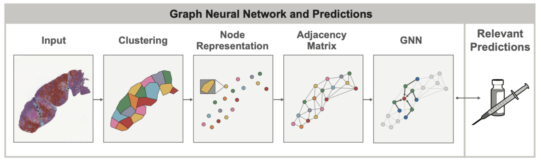
In both healthy and diseased tissue, the spatial arrangement and structure of cells can oftentimes be as important as the cells themselves. For example, when assessing lung cancers, pathologists try to look at the overall grouping and structure of tumor cells (do they form solid sheets? Or do they occur in smaller, localized clusters?) to determine if the cancer belongs to specific subtypes which can have vastly different prognosis. Such spatial relationships between cells and other tissue structures can be modeled using graphs to capture tissue topology and cellular composition at the same time. Graph Neural Networks (GNNs) allow learning spatial patterns within these graphs that relate to other clinical variables, for example overexpression of genes in certain cancers.

In late 2020, when PathAI started using GNNs on tissue samples, PyTorch had the best and most mature support for GNN functionality via the PyG package. This made PyTorch the natural choice for our team given that GNN models were something that we knew would be an important ML concept we wanted to explore. 

One of the main value-adds of GNN’s in the context of tissue samples is that the graph itself can uncover spatial relationships that would otherwise be very difficult to find by visual inspection alone. In our recent AACR publication, we showed that by using GNNs, we can better understand the way the presence of immune cell aggregates (specifically tertiary lymphoid structures, or TLS) in the tumor microenvironment can influence patient prognosis. In this case, the GNN approach was used to predict expression of genes associated with the presence of TLS, and identify histological features beyond the TLS region itself that are relevant to TLS. Such insights into gene expression are difficult to identify from tissue sample images when unassisted by ML models. 

One of the most promising GNN variations we have had success with is self attention graph pooling. Let’s take a look at how we define our Self Attention Graph Pooling (SAGPool) model using PyTorch and PyG:

class SAGPool(torch.nn.Module):
  def __init__(self, ...):
    super().__init__()
    self.conv1 = GraphConv(in_features, hidden_features, aggr='mean')
    self.convs = torch.nn.ModuleList()
    self.pools = torch.nn.ModuleList()
    self.convs.extend([GraphConv(hidden_features, hidden_features, aggr='mean') for i in range(num_layers - 1)])
    self.pools.extend([SAGPooling(hidden_features, ratio, GNN=GraphConv, min_score=min_score) for i in range((num_layers) // 2)])
    self.jump = JumpingKnowledge(mode='cat')
    self.lin1 = Linear(num_layers * hidden_features, hidden_features)
    self.lin2 = Linear(hidden_features, out_features)
    self.out_activation = out_activation
    self.dropout = dropout

In the above code, we begin by defining a single convolutional graph layer and then add two module list layers which allow us to pass in a variable number of layers. We then take our empty module list and append a variable number of GraphConv layers followed by a variable number of SAGPooling layers. We finish up our SAGPool definition by adding a JumpingKnowledge Layer, two linear layers, our activation function, and our dropout value. PyTorch’s intuitive syntax allows us to abstract away the complexity of working with state of the art methods like SAG Poolings while also maintaining the common approach to model development we are familiar with.

Models like our SAG Pool one described above are just one example of how GNNs with PyTorch are allowing us to explore new and novel ideas. We also recently explored multimodal CNN – GNN hybrid models which ended up being 20% more accurate than traditional Pathologist consensus scores. These innovations and interplay between traditional CNNs and GNNs are again enabled by the short research to production model development loop.

Improving Patient Outcomes

In order to achieve our mission of improving patient outcomes with AI-powered pathology, PathAI needs to rely on an ML development framework that (1) facilitates quick iteration and easy extension (i.e. Model configuration as code) during initial phases of development and exploration (2) scales model training and inference to massive images (3) easily and robustly serves models for production uses of our products (in clinical trials and beyond). As we’ve demonstrated, PyTorch offers us all of these capabilities and more. We are incredibly excited about the future of PyTorch and cannot wait to see what other impactful challenges we can solve using the framework.

A BetterTransformer for Fast Transformer Inference

12 Jul 2022, 1:25 am

tl;dr Transformers achieve state-of-the-art performance for NLP, and are becoming popular for a myriad of other tasks. They are computationally expensive which has been a blocker to their widespread productionisation. Launching with PyTorch 1.12, BetterTransformer implements a backwards-compatible fast path of torch.nn.TransformerEncoder for Transformer Encoder Inference and does not require model authors to modify their models. BetterTransformer improvements can exceed 2x in speedup and throughput for many common execution scenarios. To use BetterTransformer, install PyTorch 1.12 and start using high-quality, high-performance Transformer models with the PyTorch API today.

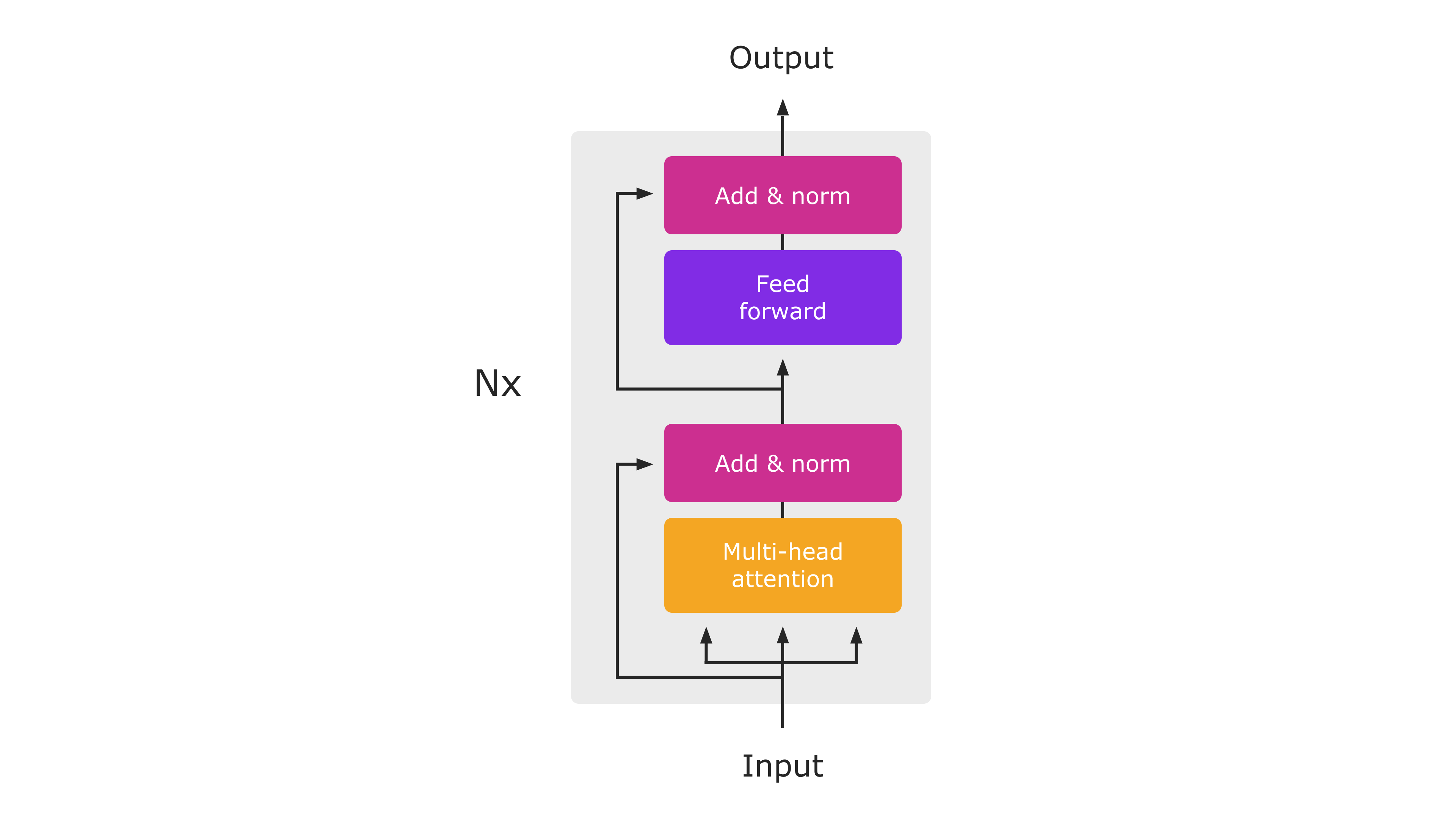
Diagram of the Transformer Encoder Architecture (from “Attention Is All You Need“). During Inference, the entire module will execute as a single PyTorch-native function.

In this blog post, we share the following topics — Performance Improvements, Backwards compatibility, and Taking advantage of the FastPath. Learn more about these topics below.

Performance Improvements

BetterTransformer launches with accelerated native implementations of MultiHeadAttention and TransformerEncoderLayer for CPUs and GPUs. These fast paths are integrated in the standard PyTorch Transformer APIs, and will accelerate TransformerEncoder, TransformerEncoderLayer and MultiHeadAttention nn.modules. These new modules implement two types of optimizations: (1) fused kernels combine multiple individual operators normally used to implement Transformers to provide a more efficient implementation, and (2) take advantage of sparsity in the inputs to avoid performing unnecessary operations on padding tokens. Padding tokens frequently account for a large fraction of input batches in many Transformer models used for Natural Language Processing.

Backwards compatibility

Advantageously, no model changes are necessary to benefit from the performance boost offered by BetterTransformer. To benefit from fast path execution, inputs and operating conditions must satisfy some access conditions (see below). While the internal implementation of Transformer APIs has changed, PyTorch 1.12 maintains strict compatibility with Transformer modules shipped in previous versions, enabling PyTorch users to use models created and trained with previous PyTorch releases while benefiting from BetterTransformer improvements.

In addition to enabling the PyTorch nn.Modules, BetterTransformer provides improvements for PyTorch libraries. Performance benefits will become available through two different enablement paths:

1. Transparent acceleration: Current users of PyTorch nn.Modules such as MultiHeadAttention as well as higher-level Transformer components will benefit from the improved performance of the new nn.Modules automatically. An example of this is the visual transformer (ViT) implementation used in the torchvision library (code link).
2. Torchtext library acceleration: As part of this project, we have optimized Torchtext to build on the PyTorch core API to benefit from BetterTransformer enhancements while maintaining strict and transparent compatibility with previous library versions and models trained with previous Torchtext versions. Using PyTorch Transformers in Torchtext also ensures that Torchtext will benefit from expected future enhancements to the PyTorch Transformer implementation.

Taking advantage of the Fastpath

BetterTransformer is a fastpath for the PyTorch Transformer API. The fastpath is a native, specialized implementation of key Transformer functions for CPU and GPU that applies to common Transformer use cases.

To take advantage of input sparsity (i.e. padding) in accelerating your model (see Figure 2), set the keyword argument enable_nested_tensor=True when instantiating a TransformerEncoder and pass in the src_key_padding_mask argument (which denotes padding tokens) during inference. This requires the padding mask to be contiguous, which is the typical case.

Currently, the BetterTransformer speedup only applies to transformer encoder models used in inference. To benefit from fastpath execution, models must be composed of any of the following components: TransformerEncoder, TransformerEncoderLayer or MultiheadAttention (MHA). Fastpath execution is also subject to some criteria. Most importantly, the model must be executed in inference mode and operate on input tensors that do not collect gradient tape information (e.g., running with torch.no_grad). The full list of conditions can be found at these links for nn.MultiHeadAttention and nn.TransformerEncoder, respectively. If the criteria are not met, control flows to the legacy PyTorch 1.11 Transformer implementation which has the same API, but lacks the fastpath performance boost.

Other transformer models (such as decoder models) which use the PyTorch MultiheadAttention module will benefit from the BetterTransformer fastpath. Planned future work is to expand the end-to-end BetterTransformer fastpath to models based on TransformerDecoder to support popular seq2seq and decoder-only (e.g., OPT) model architectures, and to training.

Speedups

The following graphs show the performance achieved for the BERT-base model with small and large-scale inputs:

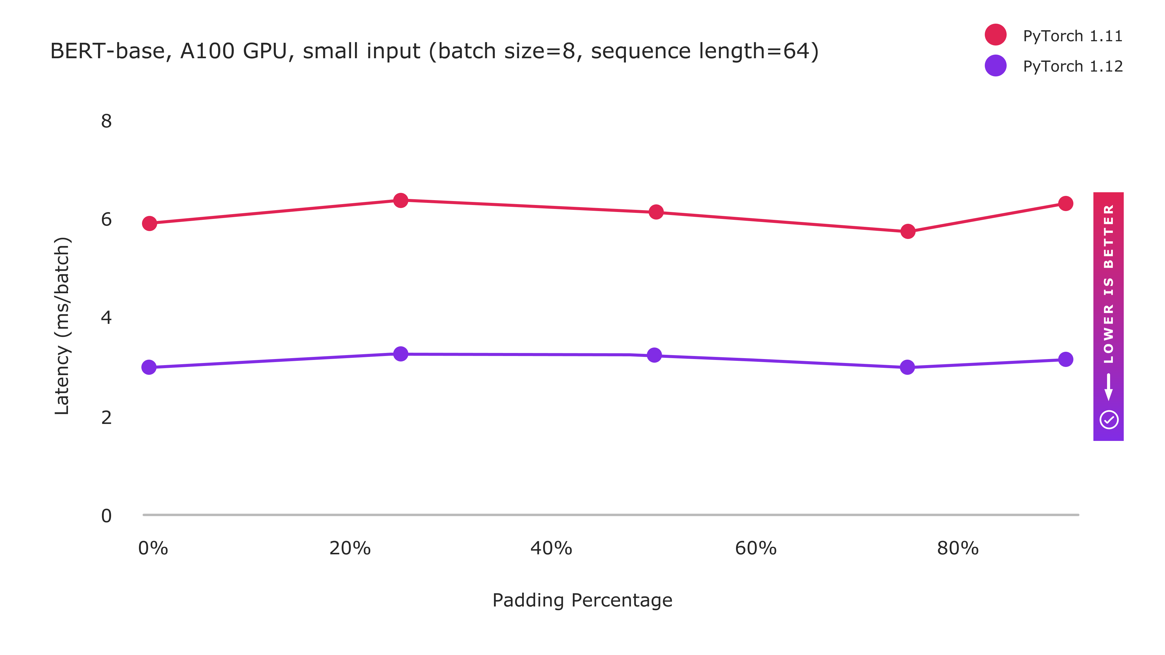
Figure 1: PyTorch 1.12 Improvements with BetterTransformer fastpath execution

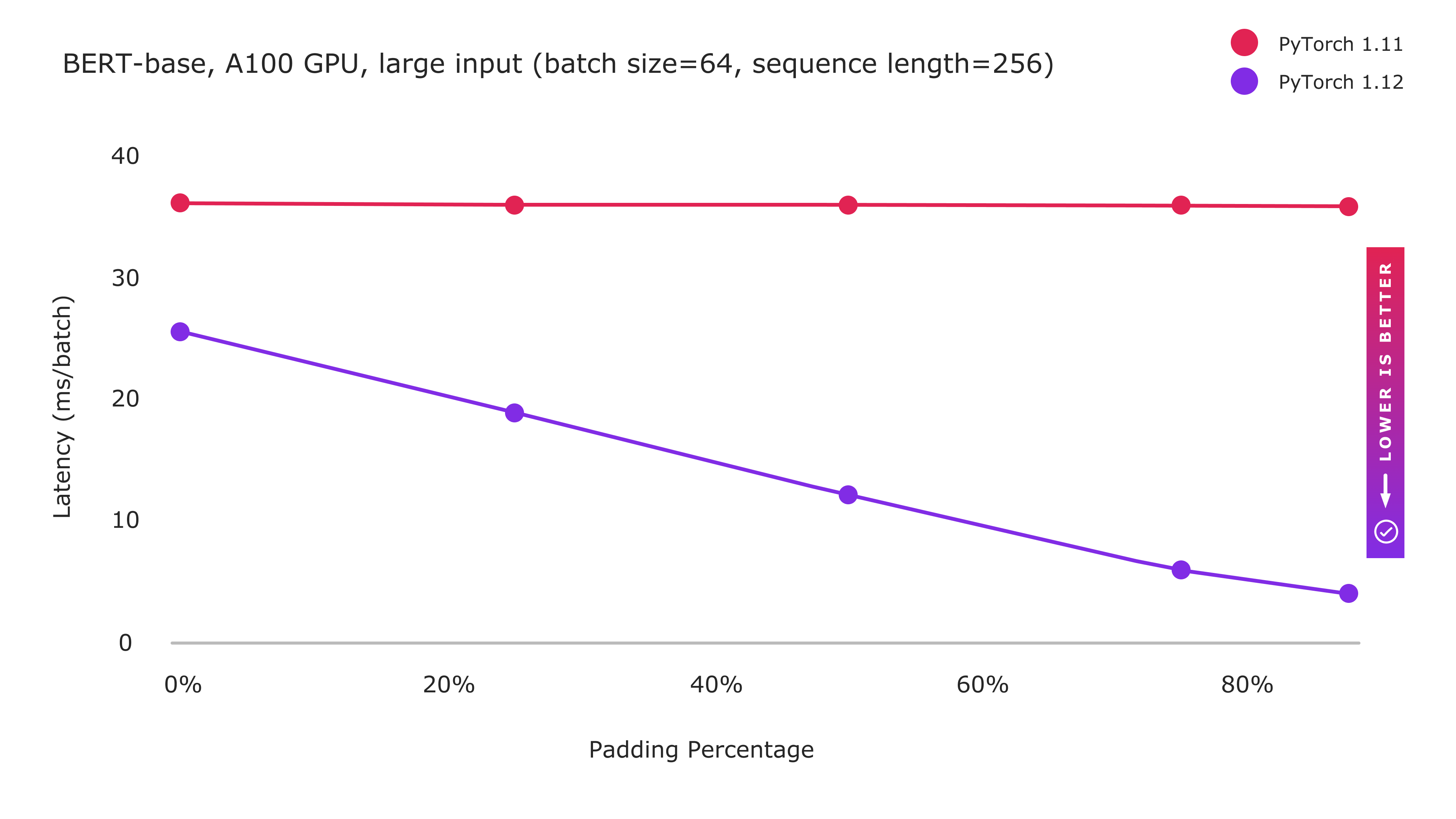
Figure 2: PyTorch 1.12 Improvements with BetterTransformer fastpath execution
with sparsity optimization enabled by enable_nested_tensor=True

BetterTransformer includes two types of optimization: (1) fused kernels implementing multiple operations more efficiently in a single kernel, and (2) exploiting sparsity by avoiding unnecessary processing on padding tokens. Enhanced performance for small input sizes benefits primarily from the fused kernel implementations, and shows a constant performance improvement regardless of padding amount. While large inputs still benefit from fused kernels, the computation heavy processing limits the benefits that may be obtained by the fused kernels as baseline performance is already closer to the theoretical peak. However, as we increase the amount of padding, performance increases dramatically as increasingly large amounts of computation can be avoided by exploiting the sparsity introduced by padding in NLP workloads.

Future Work

As part of our ongoing work on PyTorch BetterTransformer, we are working on extending BetterTransformer improvements to Transformer Decoders. We aim to expand beyond inference to training as well.

We are partnering to enable BetterTransformer on additional libraries such as FairSeq, MetaSeq, and HuggingFace to benefit all Transformer-based PyTorch models. We’ll provide future updates on the progress of BetterTransformer accelerations for the larger PyTorch ecosystem as part of this blog series.

Acknowledgements: The authors would like to thank Lin Qiao, Ajit Mathews, Andrew Tulloch, Dmytro Dzhulgakov, Natalia Gimelshein, Emad El-Haraty, Mark Saroufim, Adnan Aziz, Geeta Chauhan, and Hamid Shojanazeri for their support, contributions and many helpful suggestions throughout the course of this project, and in the preparation of this blog.

Crayon boosts speed, accuracy of healthcare auditing process using Azure Machine Learning and PyTorch

28 Jun 2022, 5:32 am

Healthcare providers need to be able to verify that they’re maintaining the highest operating safety and efficacy standards. Those standards are set by a national accreditation organization whose surveyors, often healthcare professionals themselves, regularly visit facilities and document situations that might need to be corrected or brought back in line with the latest rules and policies. That assessment and accreditation process generates a huge amount of data, and even the most experienced

PyTorch 1.12: TorchArrow, Functional API for Modules and nvFuser, are now available

28 Jun 2022, 4:30 am

We are excited to announce the release of PyTorch 1.12 (release note)! This release is composed of over 3124 commits, 433 contributors. Along with 1.12, we are releasing beta versions of AWS S3 Integration, PyTorch Vision Models on Channels Last on CPU, Empowering PyTorch on Intel® Xeon® Scalable processors with Bfloat16 and FSDP API. We want to sincerely thank our dedicated community for your contributions.

Summary:

• Functional APIs to functionally apply module computation with a given set of parameters
• Complex32 and Complex Convolutions in PyTorch
• DataPipes from TorchData fully backward compatible with DataLoader
• functorch with improved coverage for APIs
• nvFuser a deep learning compiler for PyTorch
• Changes to float32 matrix multiplication precision on Ampere and later CUDA hardware
• TorchArrow, a new beta library for machine learning preprocessing over batch data

Frontend APIs

Introducing TorchArrow

We’ve got a new Beta release ready for you to try and use: TorchArrow. This is a library for machine learning preprocessing over batch data. It features a performant and Pandas-style, easy-to-use API in order to speed up your preprocessing workflows and development.

Currently, it provides a Python DataFrame interface with the following features:

• High-performance CPU backend, vectorized and extensible User-Defined Functions (UDFs) with Velox
• Seamless handoff with PyTorch or other model authoring, such as Tensor collation and easily plugging into PyTorch DataLoader and DataPipes
• Zero copy for external readers via Arrow in-memory columnar format

For more details, please find our 10-min tutorial, installation instructions, API documentation, and a prototype for data preprocessing in TorchRec.

(Beta) Functional API for Modules

PyTorch 1.12 introduces a new beta feature to functionally apply Module computation with a given set of parameters. Sometimes, the traditional PyTorch Module usage pattern that maintains a static set of parameters internally is too restrictive. This is often the case when implementing algorithms for meta-learning, where multiple sets of parameters may need to be maintained across optimizer steps.

The new torch.nn.utils.stateless.functional_call() API allows for:

• Module computation with full flexibility over the set of parameters used
• No need to reimplement your module in a functional way
• Any parameter or buffer present in the module can be swapped with an externally-defined value for use in the call. Naming for referencing parameters / buffers follows the fully-qualified form in the module’s state_dict()

Example:

import torch
from torch import nn
from torch.nn.utils.stateless import functional_call

class MyModule(nn.Module):
    def __init__(self):
        super().__init__()
        self.fc1 = nn.Linear(3, 3)
        self.bn = nn.BatchNorm1d(3)
        self.fc2 = nn.Linear(3, 3)

    def forward(self, x):
        return self.fc2(self.bn(self.fc1(x)))

m = MyModule()

# Define parameter / buffer values to use during module computation.
my_weight = torch.randn(3, 3, requires_grad=True)
my_bias = torch.tensor([1., 2., 3.], requires_grad=True)
params_and_buffers = {
    'fc1.weight': my_weight,
    'fc1.bias': my_bias,
    # Custom buffer values can be used too.
    'bn.running_mean': torch.randn(3),
}

# Apply module computation to the input with the specified parameters / buffers.
inp = torch.randn(5, 3)
output = functional_call(m, params_and_buffers, inp)

(Beta) Complex32 and Complex Convolutions in PyTorch

PyTorch today natively supports complex numbers, complex autograd, complex modules, and numerous complex operations, including linear algebra and Fast Fourier Transform (FFT) operators. Many libraries, including torchaudio and ESPNet, already make use of complex numbers in PyTorch, and PyTorch 1.12 further extends complex functionality with complex convolutions and the experimental complex32 (“complex half”) data type that enables half precision FFT operations. Due to the bugs in CUDA 11.3 package, we recommend using CUDA 11.6 package from wheels if you are using complex numbers.

(Beta) Forward-mode Automatic Differentiation

Forward-mode AD allows the computation of directional derivatives (or equivalently, Jacobian-vector products) eagerly in the forward pass. PyTorch 1.12 significantly improves the operator coverage for forward-mode AD. See our tutorial for more information.

TorchData

BC DataLoader + DataPipe

`DataPipe` from TorchData becomes fully backward compatible with the existing `DataLoader` regarding shuffle determinism and dynamic sharding in both multiprocessing and distributed environments.

(Beta) AWS S3 Integration

DataPipes based on AWSSDK have been integrated into TorchData. It provides the following features backed by native AWSSDK:

• Retrieve list of urls from each S3 bucket based on prefix
  • Support timeout to prevent hanging indefinitely
  • Support to specify S3 bucket region
• Load data from S3 urls
  • Support buffered and multi-part download
  • Support to specify S3 bucket region

AWS native DataPipes are still in the beta phase. And, we will keep tuning them to improve their performance.

(Prototype) DataLoader2

DataLoader2 became available in prototype mode. We are introducing new ways to interact between DataPipes, DataLoading API, and backends (aka ReadingServices). Feature is stable in terms of API, but functionally not complete yet. We welcome early adopters and feedback, as well as potential contributors.

For more details, please checkout the link.

functorch

Inspired by Google JAX, functorch is a library that offers composable vmap (vectorization) and autodiff transforms. It enables advanced autodiff use cases that would otherwise be tricky to express in PyTorch. Examples of these include:

• running ensembles of models on a single machine
• efficiently computing Jacobians and Hessians
• computing per-sample-gradients (or other per-sample quantities)

We’re excited to announce functorch 0.2.0 with a number of improvements and new experimental features.

Significantly improved coverage

We significantly improved coverage for functorch.jvp (our forward-mode autodiff API) and other APIs that rely on it (functorch.{jacfwd, hessian}).

(Prototype) functorch.experimental.functionalize

Given a function f, functionalize(f) returns a new function without mutations (with caveats). This is useful for constructing traces of PyTorch functions without in-place operations. For example, you can use make_fx(functionalize(f)) to construct a mutation-free trace of a pytorch function. To learn more, please see the documentation.

For more details, please see our installation instructions, documentation, tutorials, and release notes.

Performance Improvements

Introducing nvFuser, a deep learning compiler for PyTorch

In PyTorch 1.12, Torchscript is updating its default fuser (for Volta and later CUDA accelerators) to nvFuser, which supports a wider range of operations and is faster than NNC, the previous fuser for CUDA devices. A soon to be published blog post will elaborate on nvFuser and show how it speeds up training on a variety of networks.

See the nvFuser documentation for more details on usage and debugging.

Changes to float32 matrix multiplication precision on Ampere and later CUDA hardware

PyTorch supports a variety of “mixed precision” techniques, like the torch.amp (Automated Mixed Precision) module and performing float32 matrix multiplications using the TensorFloat32 datatype on Ampere and later CUDA hardware for faster internal computations. In PyTorch 1.12 we’re changing the default behavior of float32 matrix multiplications to always use full IEEE fp32 precision, which is more precise but slower than using the TensorFloat32 datatype for internal computation. For devices with a particularly high ratio of TensorFloat32 to float32 throughput such as A100, this change in defaults can result in a large slowdown.

If you’ve been using TensorFloat32 matrix multiplications then you can continue to do so by setting torch.backends.cuda.matmul.allow_tf32 = True

which is supported since PyTorch 1.7. Starting in PyTorch 1.12 the new matmul precision API can be used, too: torch.set_float32_matmul_precision(“highest”|”high”|”medium”)

To reiterate, PyTorch’s new default is “highest” precision for all device types. We think this provides better consistency across device types for matrix multiplications. Documentation for the new precision API can be found here. Setting the “high” or “medium” precision types will enable TensorFloat32 on Ampere and later CUDA devices. If you’re updating to PyTorch 1.12 then to preserve the current behavior and faster performance of matrix multiplications on Ampere devices, set precision to “high”.

Using mixed precision techniques is essential for training many modern deep learning networks efficiently, and if you’re already using torch.amp this change is unlikely to affect you. If you’re not familiar with mixed precision training then see our soon to be published “What Every User Should Know About Mixed Precision Training in PyTorch” blogpost.

(Beta) Accelerating PyTorch Vision Models with Channels Last on CPU

Memory formats have a significant impact on performance when running vision models, generally Channels Last is more favorable from a performance perspective due to better data locality. 1.12 includes fundamental concepts of memory formats and demonstrates performance benefits using Channels Last on popular PyTorch vision models on Intel® Xeon® Scalable processors.

• Enables Channels Last memory format support for the commonly used operators in CV domain on CPU, applicable for both inference and training
• Provides native level optimization on Channels Last kernels from ATen, applicable for both AVX2 and AVX512
• Delivers 1.3x to 1.8x inference performance gain over Channels First for TorchVision models on Intel® Xeon® Ice Lake (or newer) CPUs

(Beta) Empowering PyTorch on Intel® Xeon® Scalable processors with Bfloat16

Reduced precision numeric formats like bfloat16 improves PyTorch performance across multiple deep learning training workloads. PyTorch 1.12 includes the latest software enhancements on bfloat16 which applies to a broader scope of user scenarios and showcases even higher performance gains. The main improvements include:

• 2x hardware compute throughput vs. float32 with the new bfloat16 native instruction VDPBF16PS, introduced on Intel® Xeon® Cooper Lake CPUs
• 1/2 memory footprint of float32, faster speed for memory bandwidth intensive operators
• 1.4x to 2.2x inference performance gain over float32 for TorchVision models on Intel® Xeon® Cooper Lake (or newer) CPUs

(Prototype) Introducing Accelerated PyTorch Training on Mac

With the PyTorch 1.12 release, developers and researchers can now take advantage of Apple silicon GPUs for significantly faster model training. This unlocks the ability to perform machine learning workflows like prototyping and fine-tuning locally, right on Mac. Accelerated GPU training is enabled using Apple’s Metal Performance Shaders (MPS) as a backend. The benefits include performance speedup from accelerated GPU training and the ability to train larger networks or batch sizes locally. Learn more here.

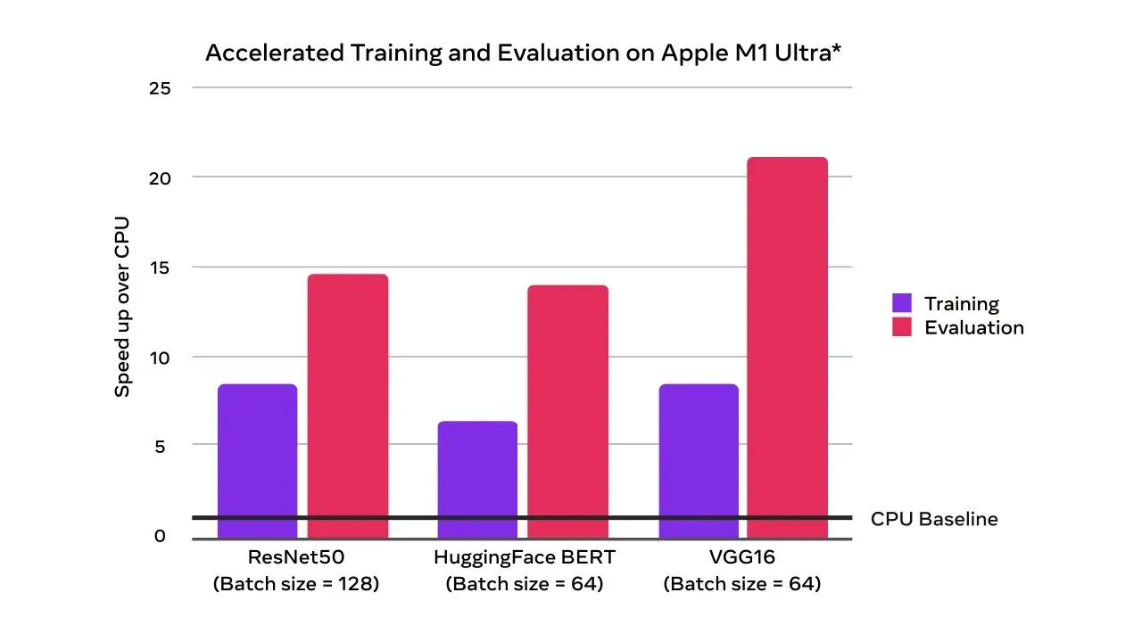
Accelerated GPU training and evaluation speedups over CPU-only (times faster)

Alongside the new MPS device support, the M1 binaries for Core and Domain libraries that have been available for the last few releases are now an official prototype feature. These binaries can be used to run PyTorch natively on Apple Silicon.

(Prototype) BetterTransformer: Fastpath execution for Transformer Encoder Inference

PyTorch now supports CPU and GPU fastpath implementations (“BetterTransformer”) for several Transformer Encoder modules including TransformerEncoder, TransformerEncoderLayer, and MultiHeadAttention (MHA). The BetterTransformer fastpath architecture Better Transformer is consistently faster – 2x for many common execution scenarios, depending on model and input characteristics. The new BetterTransformer-enabled modules are API compatible with previous releases of the PyTorch Transformer API and will accelerate existing models if they meet fastpath execution requirements, as well as read models trained with previous versions of PyTorch. PyTorch 1.12 includes:

• BetterTransformer integration for Torchtext’s pretrained RoBERTa and XLM-R models
• Torchtext which builds on the PyTorch Transformer API
• Fastpath execution for improved performance by reducing execution overheads with fused kernels which combines multiple operators into a single kernel
• Option to achieve additional speedups by taking advantage of data sparsity during the processing of padding tokens in natural-language processing (by setting enable_nested_tensor=True when creating a TransformerEncoder)
• Diagnostics to help users understand why fastpath execution did not occur

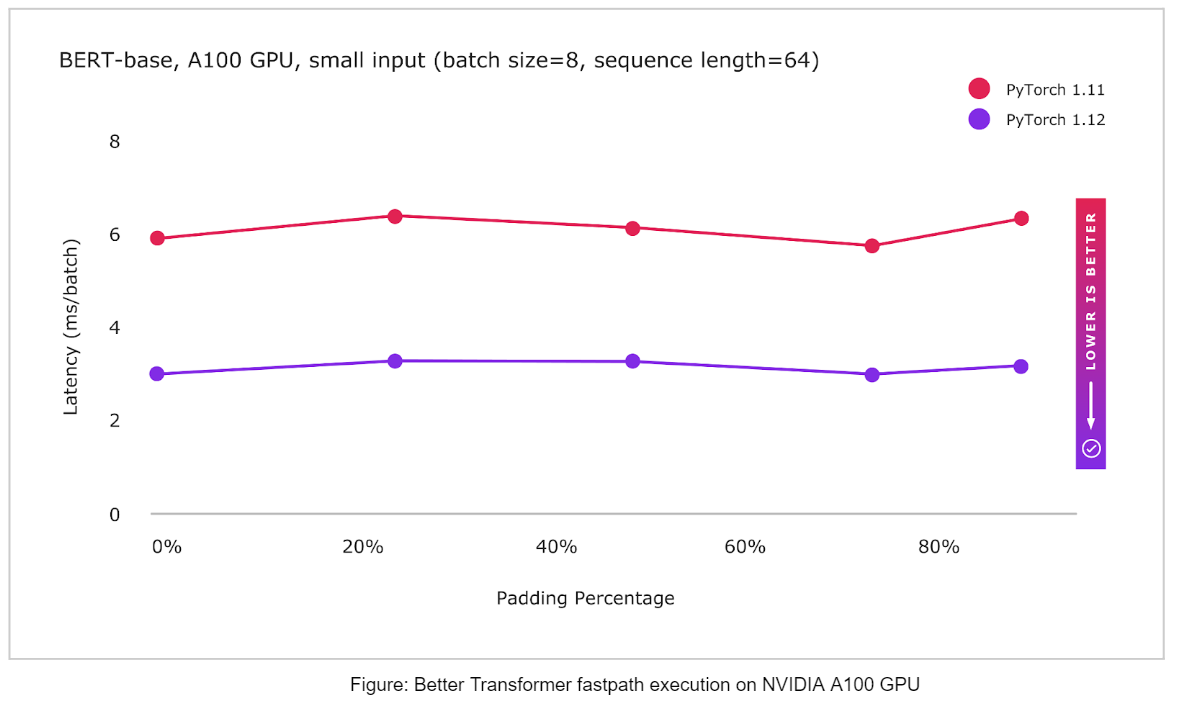
Distributed

(Beta) Fully Sharded Data Parallel (FSDP) API

FSDP API helps easily scale large model training by sharding a model’s parameters, gradients and optimizer states across data parallel workers while maintaining the simplicity of data parallelism. The prototype version was released in PyTorch 1.11 with a minimum set of features that helped scaling tests of models with up to 1T parameters.

In this beta release, FSDP API added the following features to support various production workloads. Highlights of the the newly added features in this beta release include:

1. Universal sharding strategy API – Users can easily change between sharding strategies with a single line change, and thus compare and use DDP (only data sharding), FSDP (full model and data sharding), or Zero2 (only sharding of optimizer and gradients) to optimize memory and performance for their specific training needs
2. Fine grained mixed precision policies – Users can specify a mix of half and full data types (bfloat16, fp16 or fp32) for model parameters, gradient communication, and buffers via mixed precision policies. Models are automatically saved in fp32 to allow for maximum portability
3. Transformer auto wrapping policy – allows for optimal wrapping of Transformer based models by registering the models layer class, and thus accelerated training performance
4. Faster model initialization using device_id init – initialization is performed in a streaming fashion to avoid OOM issues and optimize init performance vs CPU init
5. Rank0 streaming for full model saving of larger models – Fully sharded models can be saved by all GPU’s streaming their shards to the rank 0 GPU, and the model is built in full state on the rank 0 CPU for saving

For more details and example code, please checkout the documentation and the tutorial.

Thanks for reading, If you’re interested in these updates and want to join the PyTorch community, we encourage you to join the discussion forums and open GitHub issues. To get the latest news from PyTorch, follow us on Twitter, Medium, YouTube, and LinkedIn.

Cheers!

Team PyTorch